Vaex is an incredibly powerful DataFrame library in Python capable of processing hundreds of millions or even billions of rows per second, without loading the entire dataset in memory. This makes it particularly useful for exploration, visualization and statistical analysis of large datasets that exceed the available RAM of a single machine.

However, it is not all just about speed, but also about convenience and ease of use. In this article, we will go over 8 powerful and convenient features that will make your data analysis workflow much more efficient.

1. Lazily open and work with huge CSV files

Since its conception, Vaex was able to work with files much larger than available RAM, in a very efficient way. In fact, that is the goal of the library: to allow you to easily work with arbitrarily large datasets on commodity hardware. In the past this was only possible with binary file formats such as HDF5, Arrow and Parquet.

However, since Vaex version 4.14.0, it is possible to lazily open and work with CSV files just as easy as with the binary file formats mentioned above. This is in part thanks to the Apache Arrow project that provides a rather efficient CSV reader. Let's see how this works in practice.

print('Check file size on disk:')
!du -h /data/jovan/data/chicago-taxi/chicago_taxi_2013_2020.csv
print()

df = vaex.open('/data/jovan/data/chicago-taxi/chicago_taxi_2013_2020.csv')

print(f'Number of rows: {df.shape[0]:,}')
print(f'Number of columns: {df.shape[1]}')

mean_tip_amount = df.tip_amount.mean(progress='widget')
print(f'Mean tip amount: {mean_tip_amount:.2f}')

df.fare_amount.viz.histogram(shape=128, figsize=(6, 4), limits=[0, 42], progress='widget');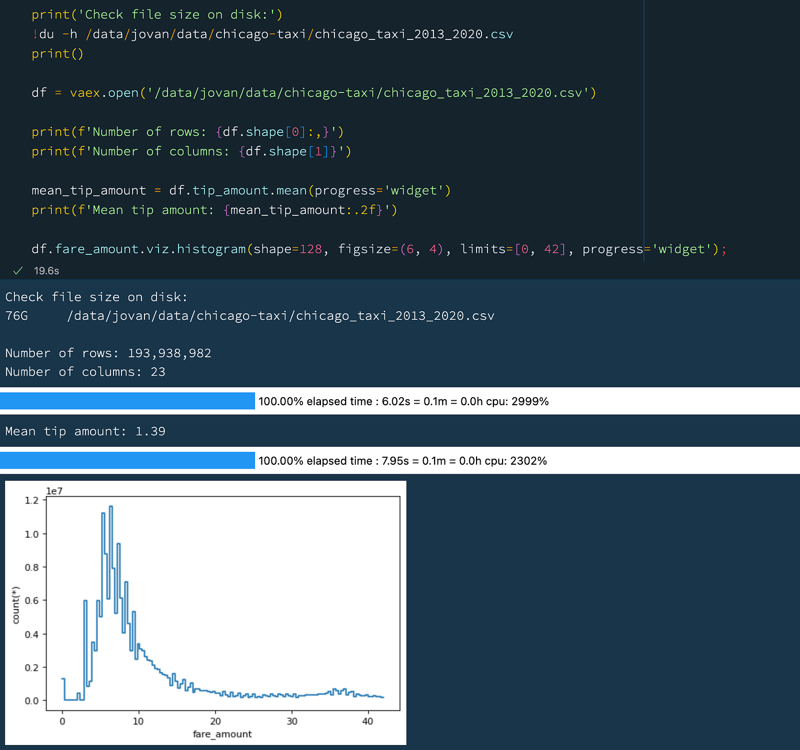

Opening and working with a 76 GB CSV file.

The above example shows how you can easily work with a rather large CSV file. Let us describe the above example in a bit more detail:

• When we use vaex.open() with a CSV file, Vaex will stream over the entire CSV file to determine the number of rows and columns, as well as the data type of each column. While this does not take any significant amount of RAM, it might take some time, depending on the number of rows and columns of the CSV. One can control how thoroughly Vaex reads the file is via the schema_infer_fraction argument. A lower numbers will result in a faster reading, but data type inference might be less accurate - it all depends on the content of the CSV file. In the above example we read through 76 GB CSV file comprised of just under 200 million rows and 23 columns in about 5 seconds with the default parameters.
• Then we calculated the mean of tip_amount column, which took 6 seconds.
• Finally we plotted a histogram fo the tip_amount column, which took 8 seconds.

Overall we read through the entire 76 GB CSV file 3 times in under 20 seconds, without the need to load the entire file in memory.

Also notice that the API and general behavior of Vaex is the same, regardless of the file format. This means that you can easily switch between CSV, HDF5, Arrow and Parquet files, without having to change your code.

Of course, using CSV files is suboptimal in terms of performance, and it should be generally avoided for variety of reasons. Still, large CSV files do pop up in the wild, which makes this feature quite convenient for quick checks and explorations of their contents, as well as for efficient conversions to more suitable file formats.

2. Group-by aggregations

The group-by is one of the most common operations in data analysis and needs no special introduction. There are two main ways to specify the aggregation operations in Vaex:

• Option 1: Specify the column one wants to aggregate, and the alias of the aggregation operation. The resulting column will have the same name as the input column.
• Option 2: Specify the name of the output column, and then explicitly specify the vaex aggregation method.

Let's see how this works in practice. Note that for the rest of this article we will be using a subset of the NYC Taxi dataset that contains well over 1 billion rows!

df = vaex.open('/data/yellow_taxi_2009_2015_f32.hdf5')

print(f'Number of rows: {df.shape[0]:,}')
print(f'Number of columns: {df.shape[1]}')


df.groupby(df.vendor_id, progress='widget').agg(
    {'fare_amount': 'mean',                              # Option 1
     'tip_amount_mean': vaex.agg.mean(df.tip_amount),    # Option 2
    })

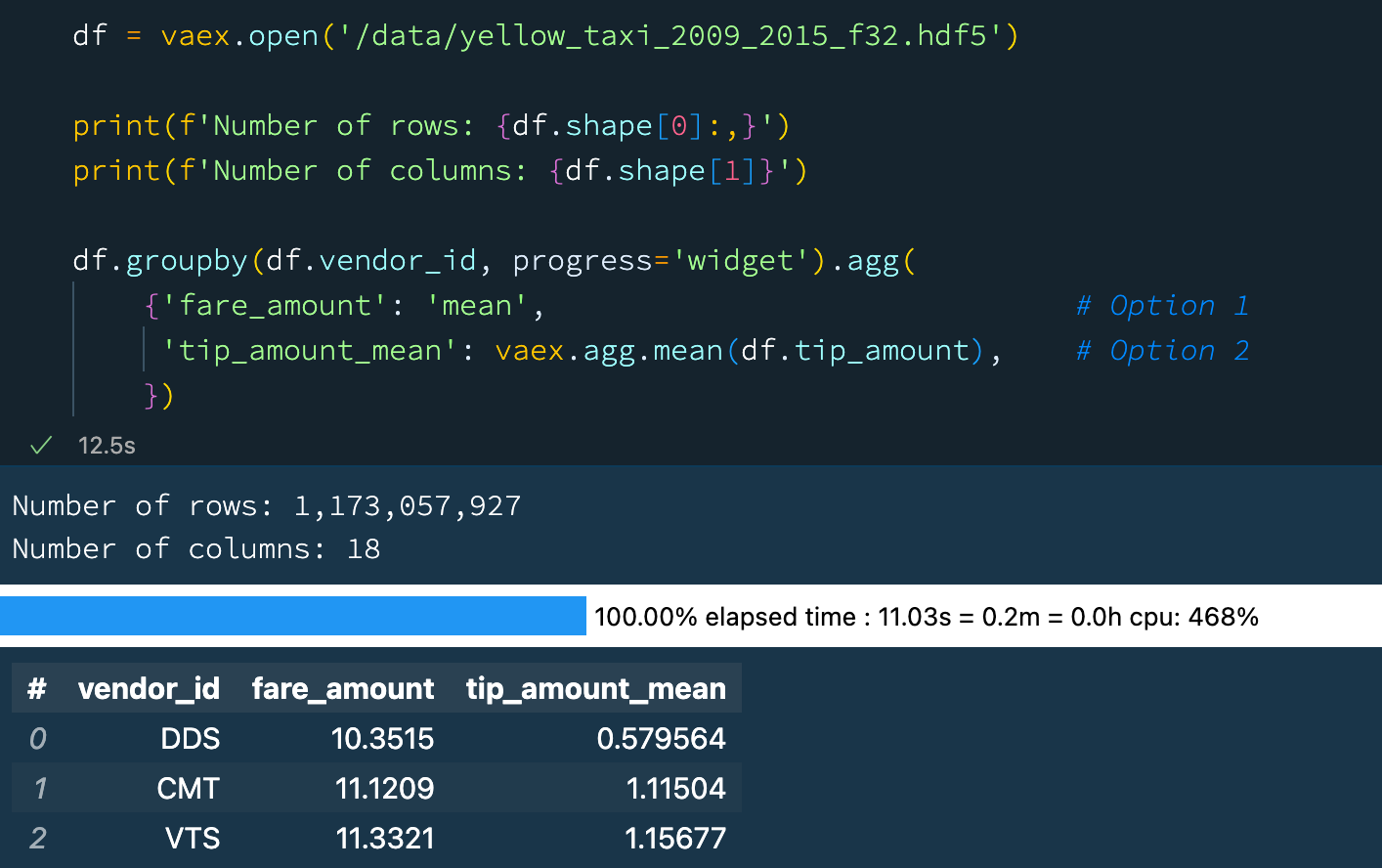Group-by aggregation with Vaex.

The above example is pretty standard. In fact many DataFrame libraries have a similar syntax. What is great about Vaex, is that the 2nd option allows one to create a linear combination of aggregators. For example:

df.groupby(df.vendor_id, progress='widget').agg(
    {'fare_amount_norm': vaex.agg.mean(df.fare_amount) / vaex.agg.std(df.fare_amount)}
    )

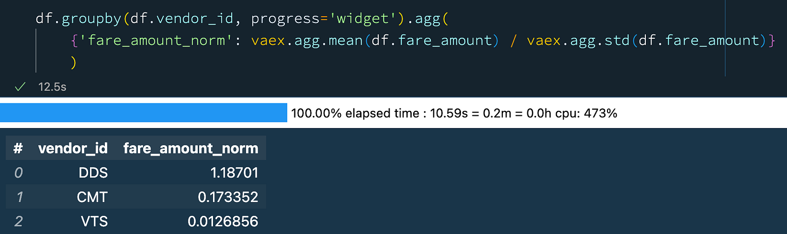Group-by aggregation with Vaex: combining aggregators.

Explicitly specifying the aggregation functions (Option 2 above) has an additional benefit: it allows one to specify a selection, i.e. a subset of the data on which the aggregator will operate. This is particularly useful when one wants do a number of aggregation operations on different subsets of the data, all in the same group-by operation! For example:

df.groupby(df.vendor_id, progress='widget').agg(
    {'fare_amount_mean_all': vaex.agg.mean(df.fare_amount),
     'fare_amount_mean_pc2': vaex.agg.mean(df.fare_amount, selection=df.passenger_count == 2),
     'fare_amount_mean_pc4': vaex.agg.mean(df.fare_amount, selection=df.passenger_count == 4)}
)

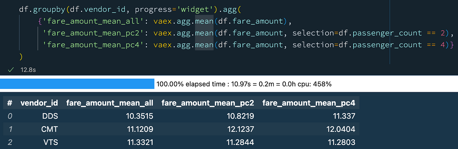Group-by aggregation with selections in Vaex.

In a single pass over the data, we calculated the mean of the "fare_amount" column for all rows, as well as for the rows where the number of passengers was 2 and 4. This is a very convenient feature! Just think about how you would do this with other DataFrame libraries or SQL. One would need to do three separate group-by aggregations, and then join the results together. Vaex simplifies this quite a bit.

3. Progress bars

When doing data analysis or writing data transformation pipelines, it is common to have various steps, some more complex then others. Thus, it is often useful to have an indication of how long each step takes, and how much time is left until the entire pipeline is finished, especially when working with rather large files. You may already have noticed that many Vaex methods support progress bars. That also is quite helpful, but we can do better! With the help of the Rich library, Vaex can provide in-depth information about the progress of each individual operation in your data transformation process. This is particularly useful to identify bottlenecks and ways to improve the performance of your code. Let's see how this looks like in practice:

with vaex.progress.tree('rich'):
    result_1 = df.groupby(df.passenger_count, agg='count')
    result_2 = df.groupby(df.vendor_id, agg=vaex.agg.sum('fare_amount'))
    result_3 = df.tip_amount.mean()

Progress tree with Vaex.

In the above example, first we want to know how many samples there are for each value of the "passenger_count" column. To do this, Vaex first calculates the set of unique "passenger_count" values and then does the aggregation for each of them. Something similar is happening in the second operation, where we want to know the total "fare_amount" for each "vendor_id". Finally we simply want to know the mean of the "tip_amount" column, which is the ratio of the sum over the number of samples of that column.

In the progress tree above, you can see the time taken for each of these steps. This makes it easy to identify bottlenecks, which is an opportunity for improvement of the data process. The progress tree also allows one to peek behind the scenes and see what operations Vaex is doing to get the result that you need.

Notice that on the right side of the progress three, there are numbers in square brackets right next to the timings.

These numbers tell which pass over the data was used for the computation

These numbers indicate the number of times Vaex needs to go over the data to calculate the result up to that specific point in the set of operations enclosed by the progress tree context manager. For example, we can see that when calculating the mean of a column, Vaex needs only one pass over the data to compute both the count and the sum of that column.

4. Async evaluations

Vaex tries to be as lazy as possible, and only evaluates expressions when it is necessary. The general guideline is that, for operations that do not change the fundamental nature of the original DataFrame, the operations are lazily evaluated. An example of this is creating new columns out of existing ones, for example combining multiple columns into a new one, or doing some kind of categorical encoding. Filtering of a DataFrame also belong to this group. Operations that change the nature of the DataFrame, such as group-by operations, or simply calculating aggregates such as the sum or a mean of a column, are eagerly evaluated. This kind of workflow provides a good balance between performance and convenience when doing interactive data exploration or analysis.

When the data transformation process or the data pipeline is well defined, one may want to optimize things with performance in mind. With the delay=True argument which is supported by many Vaex methods, one can schedule operations to be executed in parallel. This allows Vaex to build a computational graph ahead of time, and try to find the most efficient way of computing the result. Let's revisit the earlier example, but now schedule all operations to be executed simultaneously:

with vaex.progress.tree('rich'):
    result_1 = df.groupby(df.passenger_count, agg='count', delay=True)
    result_2 = df.groupby(df.vendor_id, agg=vaex.agg.sum('fare_amount'), delay=True)
    result_3 = df.tip_amount.mean(delay=True)
    df.execute()

Delayed evaluations with Vaex.

We see that by explicitly using delayed evaluations, we can improve the performance and reduce the number of times we need to go over the data. In this case, we went from 5 passes over the data to just 2 passes when using delayed evaluations, resulting in a speed up of about 30%. You can find more examples on async programming with Vaex in this guide.

5. Caching

Because of its speed, Vaex is often used as a backend for dashboards and data apps, especially those that need to crunch through large amounts of data. When using a data app, it is common that some operations are executed repeatedly on the same or similar subsets of data. For instance, users will start on the same "home page", and choose common or popular options before diving deeper into the data. In such cases, it is often useful to cache the results of the operations, so that they can be quickly retrieved when needed. This is particularly useful when the data is large, and the operations are complex. Vaex implements an advanced, granular caching mechanism, which allows one to cache the results of individual operations, which can be reused later on. The following example shows how this works:

vaex.cache.on()

with vaex.progress.tree('rich'):
    result_1 = df.passenger_count.nunique()

with vaex.progress.tree('rich'):
    result_2 = df.groupby(df.passenger_count, agg=vaex.agg.mean('trip_distance'))

Caching operations with Vaex.

Combining the caching mechanism with the delayed evaluations leads to a superb performance. It is thus no wonder why Vaex is often used as a backend for data apps.

6. Early stopping

Vaex has a rather efficient way of determining the cardinality of a column. When using the unique, nunique or groupby methods, one can also specify the limit argument. That sets the limit of the number of unique values in the column. If the limit is exceeded, Vaex can raise an exception, or return the unique values found so far.

This is particularly useful when building data apps that allow users to pick columns freely from a dataset. Instead of wasting time and resources doing a massive group-by operation that eventually can not be visualized, we can stop early and without blowing up the memory, and give a warning to a user, or automatically chose a different path for processing or visualizing the data.

In the example below, we set the limit to 100, and we tell Vaex not to raise an exception if the limit is reached, but to simply return the result, which in this case is simply the limit:

result = df.pickup_longitude.nunique(limit=100, limit_raise=False)
print(result)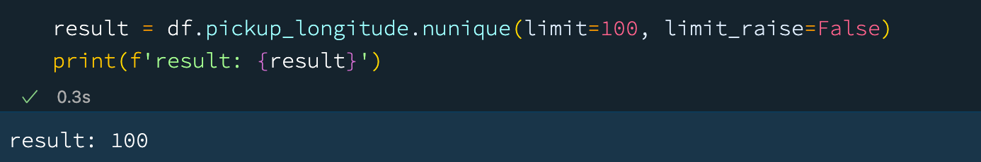

Operations limit example with Vaex.

7. Cloud support

As datasets grow, it becomes more common and practical to store them in the cloud, and keep locally only those parts of the data that we are actively working on. Vaex is quite cloud friendly - it can easily download (stream) data from any public cloud storage. More importantly, only the data that is needed will be fetched. For example when doing df.head(), only the first 5 rows will be fetched. To calculate the mean of a column, one needs all the data from that particular column, and Vaex will stream that part of the data, but it will not fetch data from any other column until it is needed. This is quite efficient and practical:

df_cloud = vaex.open('gs://vaex-data/airlines/us_airline_data_1988_2019.hdf5')

print('Size of data:')
print(f'Number of rows: {df_cloud.shape[0]:,}')
print(f'Number of columns: {df_cloud.shape[1]}')

df_cloud.head()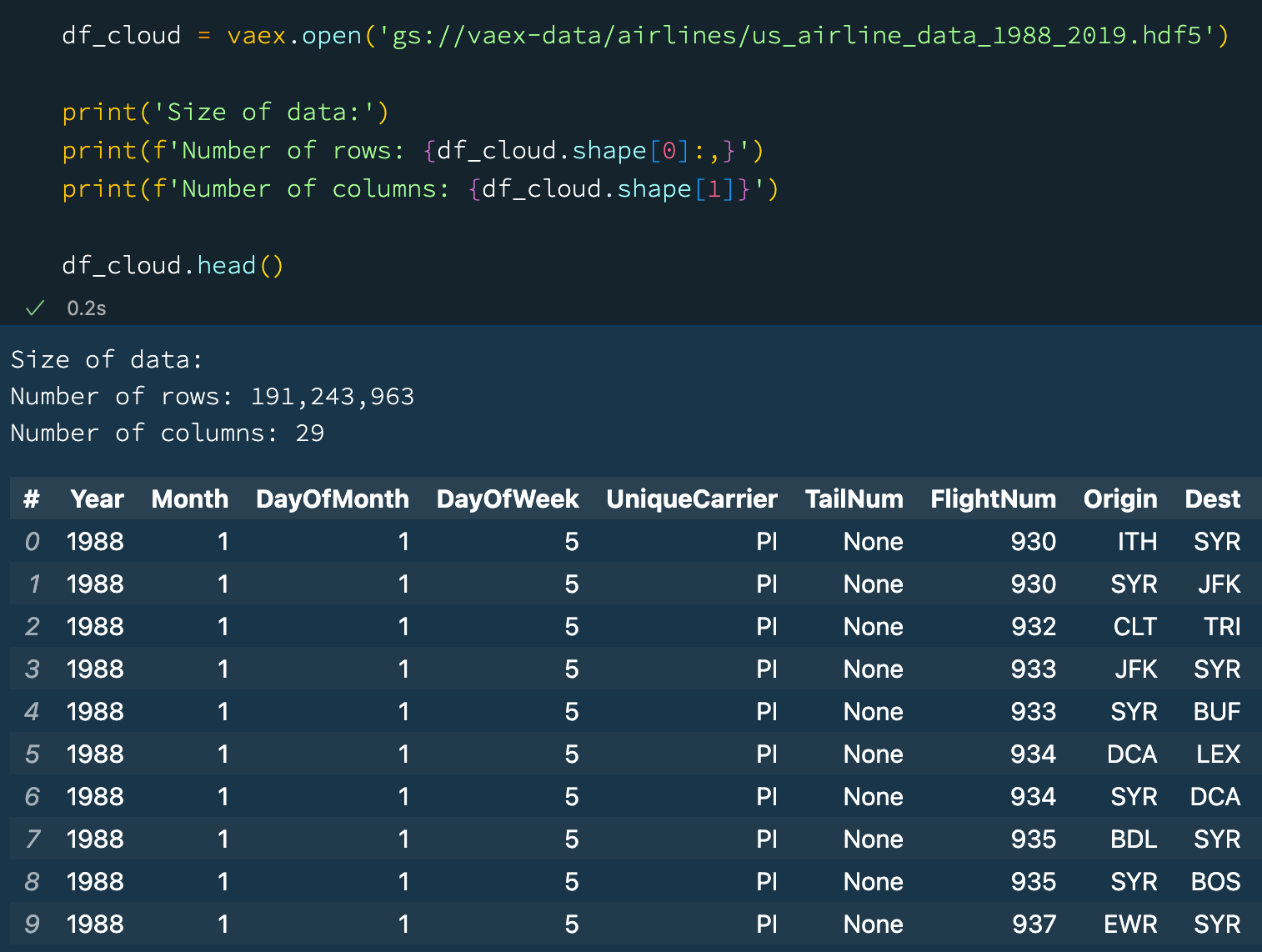

Vaex reads data directly from the Cloud.

8. Using the GPU (NVIDIA, RADEON, M1, M2)

Last but not least, did you know that Vaex can use GPUs to accelerate the evaluation of computationally expensive expressions? What is more impressive, it supports NVIDIA for Windows and Linux platforms, and Radeon and Apple Silicon for Mac OS. Data practitioners can finally take advantage of the power of the Apple Silicon devices for doing some data analysis!

In the example below we define a function that computes the arc distance between two points on a sphere. It is a rather complicated mathematical operation involving lots of trigonometry and arithmetics. Let's try to compute the mean arc distance for all taxi trips in our New York taxi dataset that comprises well over 1 billion rows:

print(f'Number of rows: {df.shape[0]:,}')

def arc_distance(theta_1, phi_1, theta_2, phi_2):
    temp = (np.sin((theta_2-theta_1)/2*np.pi/180)**2
           + np.cos(theta_1*np.pi/180)*np.cos(theta_2*np.pi/180) * np.sin((phi_2-phi_1)/2*np.pi/180)**2)
    distance = 2 * np.arctan2(np.sqrt(temp), np.sqrt(1-temp))
    return distance * 3958.8

df['arc_distance_miles_numpy'] = arc_distance(df.pickup_longitude, df.pickup_latitude,
                                              df.dropoff_longitude, df.dropoff_latitude)

# Requires cupy and NVDIA GPU
df['arc_distance_miles_cuda'] = df['arc_distance_miles_numpy'].jit_cuda()

# Requires metal2 support on MacOS (Apple Silicon and Radeon GPU supported)
# df['arc_distance_miles_metal'] = df['arc_distance_miles_numpy'].jit_metal()

result_cpu = df.arc_distance_miles_numpy.mean(progress='widget')
result_gpu = df.arc_distance_miles_cuda.mean(progress='widget')
print(f'CPU: {result_cpu:.3f} miles')
print(f'GPU: {result_gpu:.3f} miles')

Using a GPU acceleration with Vaex.

We see that using the GPU we can get a rather nice performance boost. If you do not have access to a GPU, worry not! Vaex also supports Just-In-Time compilation via Numba and Pythran which can also provide a significant performance boost.

With that last point we have come to the end of this article. I hope you will give at least some of these features a try, and I hope they will help you in your data analysis as much as they help me. Until next time!