Introduction

Training a machine learning (ML) model is often a rather lengthy and computationally intensive task, especially when using larger quantities of data.

Regardless of whether you are using your favorite deep learning framework, trusted gradient boosting machine or a custom ensemble, the model training phase can easily consume most if not all available resources on your laptop or local server, effectively "freezing" your machine and preventing you to do other tasks. Or you may not even have enough resources at hand to train a sophisticated model on all of the data you have so painstakingly gathered, or use all of the features you have so thoughtfully engineered.

On top of that, curating ML models is a continuous process: one will likely need to re-train the model relatively often to account for new data, concept drift, changes in the domain, or simply to improve the model by adjusting the input features, architecture or hyper-parameters.  Therefore, it can be rather convenient, if not necessary, to outsource the heavy lifting stage of ML model creation to a service managed by a recognized cloud provider. With this approach computational resources will not be a problem. Nowadays, one can "rent" computing instances having few hundreds of vCPUs and several Terabytes of RAM attached, or provision custom cluster configurations. In addition, one can submit multiple training jobs which will run independently and not compete with each other for resources. All this means that you can spend more of your time on creating the best model possible, and virtually no time managing, maintaining and configuring your computational resources. An important note is that such services are becoming cheaper are more accessible with time.

Google Cloud Platform & Vaex

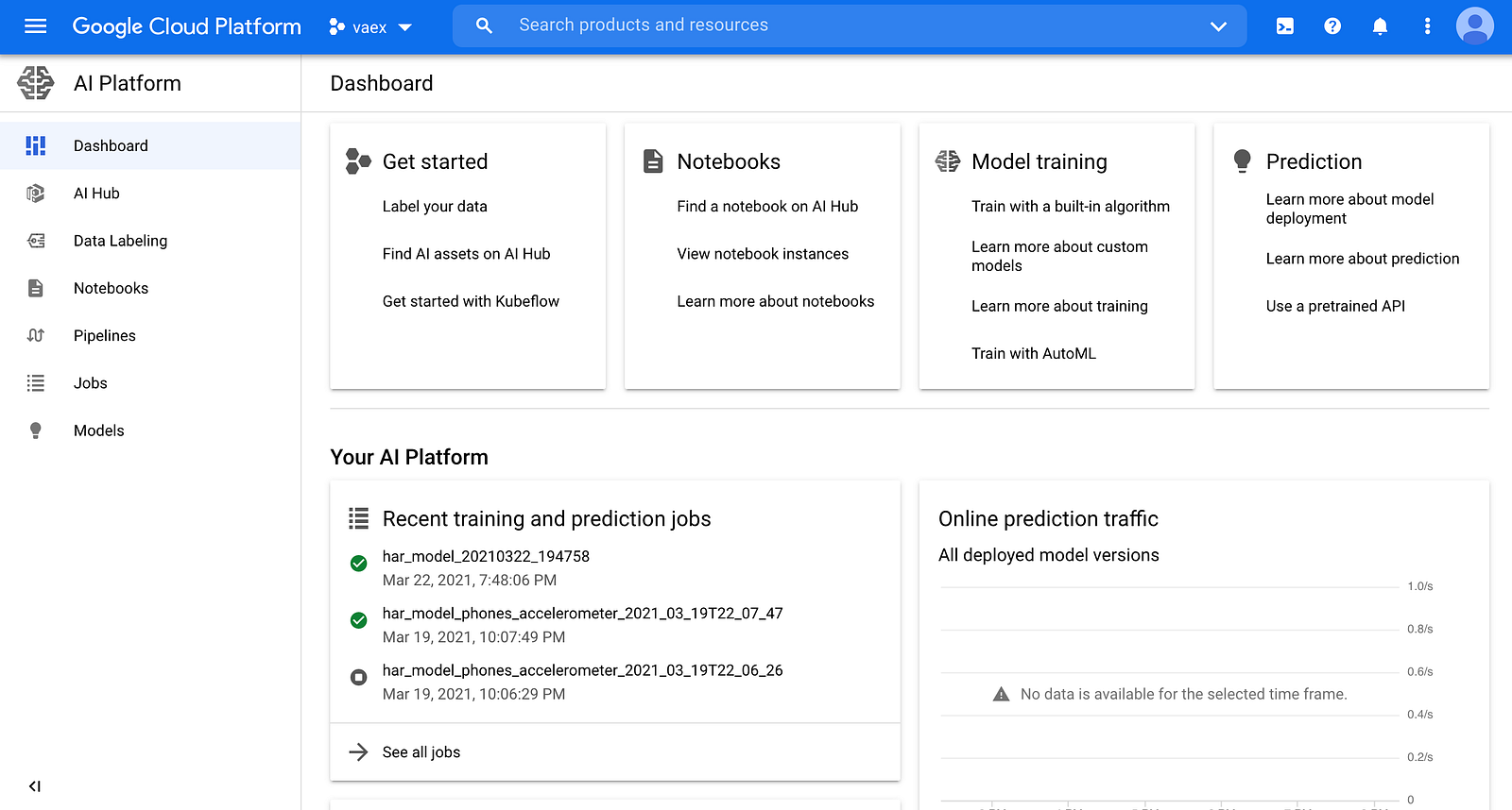The Google Cloud AI Platform seen via the Google Cloud Console

So how does Vaex fit in all of this? There are several substantial benefits to using Vaex as the core technology for building ML solutions even in cloud environments. To start with, you can host your data on a Google Cloud Storage (GCS) or an Amazon Web Services (AWS) S3 bucket, and stream it lazily to your compute instance, on a "need-to-have" basis. This means that only the specific columns that your model needs will be downloaded, and not all of the files in their entirety. One can even choose to download only a fraction of the data, which is especially useful for testing and continuous integration.

All Vaex transformations are done by fully parallelized, efficient out-of-core algorithms. That means that you always take full advantage of the compute instance you rent out, without any additional set up. The no-memory-copy policy makes it easier to choose the type of machine you require while minimizing cost without performance trade-off. 

There are a couple of more benefits that will be highlighted throughout the article. So, without further ado, let us see how one can use Vaex to build a ML solution, and how to then use GCP to make it come to life.

Before we begin

This article assumes some basic knowledge of GCP and how to interact with it through the Google Cloud Console, and via the gcloud command-line tool. If you would like to follow along with this tutorial, you will need an authenticated Google account, a GCP project, and a GCS bucket already set up. There are many useful guides in case you are not sure how to do this. If in doubt, the official GCP documentation is always a good place to start.

All the materials from this article are fully available here, along with a variety of other Vaex examples.

Creating a custom ML pipeline with Vaex

This example uses the public Heterogeneity Activity Recognition (HAR) dataset. It contains several sets of measurements captured from a group of volunteers performing one of six activities: walking, going up & down stairs, sitting, standing and biking. The measurements are captured via popular smart-phone and smart-watch devices, and comprise the triaxial acceleration and angular velocity sampled from the on-board accelerometer and gyroscope respectively. The dataset contains also the "Creation_Time" and "Arrival_Time" columns, which are the time-stamps attached to each measurement sample by the OS and mobile application respectively. The goal is to detect the particular activity performed by the wearer using just a single measurement sample. The activity itself is specified in the "gt" column which stands for "ground truth".

The following example uses the accelerometer data obtained via the smart-phone devices. It comprises just over 13 million samples. For brevity, we will not present any exploratory analysis of the data, but will jump straight into building a production ready solution. 

Let us start by creating a Python script that will fetch the data, engineer relevant features, and train and validate a model. Since we are using Vaex, fetching the data is trivial. Provided the data is in the HDF5 file format and hosted on GCS (or Amazon's S3), Vaex will lazily stream the portions that are needed for analysis. Since we already know which columns of the data are going to be needed, they can be pre-fetched right away:

log.info('Reading in the data...')
df = vaex.open('gs://vaex-data/human-activity-recognition/phones_accelerometer.hdf5')

log.info('Fetching relevant columns...')
columns_to_use = ['Arrival_Time', 'Creation_Time', 'x', 'y', 'z', 'gt']
df.nop(columns_to_use)

The next step is to randomly partition the data into 3 sets: training, validation and testing. The validation set will be used as a quality control during the training phase, while the test set will be the final, independent performance indicator on the already trained model.

log.info('Splitting the data into train, validation and test sets...')
df_train, df_val, df_test = df.split_random(into=[0.8, 0.1, 0.1], random_state=42)

At this point we can start to create some useful features. Let us begin by making a couple of coordinate transformations. We will convert the triaxial acceleration measurements from Cartesian to spherical coordinates, as well as to their "natural" coordinate system by the means of a PCA transformation:

log.info('Convert to spherical polar coordinates...')
df_train['r'] = ((df_train.x**2 + df_train.y**2 + df_train.z**2)**0.5).jit_numba()
df_train['theta'] = np.arccos(df_train.z / df_train.r).jit_numba()
df_train['phi'] = np.arctan2(df_train.y, df_train.x).jit_numba()

log.info('PCA transformation...')
df_train = df_train.ml.pca(n_components=3, features=['x', 'y', 'z'])

Even though some of the above transformations are not overly complex, we can still choose to accelerate them by using just-in-time compilation via numba. Note that we are also using the new API available in vaex-ml version 0.11, instead of the more traditional scikit-learn "fit & transform" approach. 

To capture some non-linearity in the data, we can create some feature interactions between the PCA components:

log.info('Create certain feature interactions...')
df_train['PCA_00'] = df_train.PCA_0**2
df_train['PCA_11'] = df_train.PCA_1**2
df_train['PCA_22'] = df_train.PCA_2**2

df_train['PCA_01'] = df_train.PCA_0 * df_train.PCA_1
df_train['PCA_02'] = df_train.PCA_0 * df_train.PCA_2
df_train['PCA_12'] = df_train.PCA_1 * df_train.PCA_2

Now, we will get a bit more creative. First, let us calculate the mean and standard deviation for each Principal component per activity class. Then, we will calculate the difference between the value of each Principal component and the mean of each group, scaled by the standard deviation of that group:

log.info('Calculate some summary statistics per class...')
df_summary = df_train.groupby('gt').agg({'PCA_0_mean': vaex.agg.mean('PCA_0'),
                                         'PCA_0_std': vaex.agg.std('PCA_0'),
                                         'PCA_1_mean': vaex.agg.mean('PCA_1'),
                                         'PCA_1_std': vaex.agg.std('PCA_1'),
                                         'PCA_2_mean': vaex.agg.mean('PCA_2'),
                                         'PCA_2_std': vaex.agg.std('PCA_2')
                                         }).to_pandas_df().set_index('gt')

log.info('Define features based on the summary statistics per target class...')
for class_name in df_train.gt.unique():
    feature_name = f'PCA_012_err_{class_name}'
    df_train[feature_name] = ((np.abs(df_train.PCA_0 - df_summary.loc[class_name, 'PCA_0_mean']) / df_summary.loc[class_name, 'PCA_0_std']) +
                              (np.abs(df_train.PCA_1 - df_summary.loc[class_name, 'PCA_1_mean']) / df_summary.loc[class_name, 'PCA_1_std']) +
                              (np.abs(df_train.PCA_2 - df_summary.loc[class_name, 'PCA_2_mean']) / df_summary.loc[class_name, 'PCA_2_std'])).jit_numba()

Notice how we are combining the usage of both Vaex and Pandas in creating these features. While the df_summary DataFrame will not be stored, its values are "remembered" as part of the expressions defined in the for loop that follows the groupby aggregation. The above code-block is an example of how one can very quickly and clearly create new features, without the otherwise necessary exercise of creating a custom Transformer class. 

Another interesting approach to feature engineering is to apply a clustering algorithm on subsets of already defined features, and use the resulting cluster labels as additional features. The vaex-ml package directly implements the KMeans clustering algorithm, so it is guaranteed to very fast and memory efficient. Using the KMeans algorithm, we create 3 sets of cluster labels: one by clustering the PCA components, two by clustering PCA interaction components:

logging.info('Creating kmeans clustering features using the PCA components ...')
df_train = df_train.ml.kmeans(features=['PCA_0', 'PCA_1', 'PCA_2'],
                              n_clusters=n_clusters,
                              max_iter=1000,
                              n_init=5,
                              prediction_label='kmeans_pca')

logging.info('Creating kmeans clustering features using the interacting PCA components ...')
df_train = df_train.ml.kmeans(features=['PCA_01', 'PCA_02', 'PCA_12'],
                              n_clusters=n_clusters,
                              max_iter=1000,
                              n_init=5,
                              prediction_label='kmeans_pca_inter')

logging.info('Creating kmeans clustering features using the power PCA components ...')
df_train = df_train.ml.kmeans(features=['PCA_00', 'PCA_11', 'PCA_22'],
                              n_clusters=n_clusters,
                              max_iter=1000,
                              n_init=5,
                              prediction_label='kmeans_pca_power')

In Vaex any model is treated as a transformer, so it's outputs are readily available to be used as any other features in the downstream computational graph. Finally, we can also make use of the time-stamp features, and calculate the difference between the "Arrival_Time" and "Creation_Time" columns, to which we apply standard scaling:

log.info('Create time feature...')
df_train['time_delta'] = df_train.Arrival_Time - df_train.Creation_Time
df_train = df_train.ml.max_abs_scaler(features=['time_delta'], prefix='scaled_')

Once we are done defining all the features, we can gather them into a single list for convenience:

log.info('Gather all the features that will be used for training the model...')
features = df_train.get_column_names(regex='x|y|z|r|theta|phi|PCA_|scaled_|kmeans_')

The last part of the data preparation is to encode the target column "gt" into a numeric format. Following the encoding, we will also define a inverse mapping dictionary, which we will later use to translate the predicted classes to their true labels.

log.info('Encoding the target variable...')
target_encoder = df_train.ml.label_encoder(features=['gt'], prefix='enc_', transform=False)
df_train = target_encoder.transform(df_train)
target_mapper_inv = {key: value for value, key in target_encoder.labels_['gt'].items()}

At this point, we are finally ready to start training the model. You may have noticed that we have not bothered to explicitly create a pipeline to allow for all the data transformations to be propagated to the validation and test sets. This is because a Vaex DataFrame implicitly keeps record of all the transformations and modifications done to the data. Filters, categorical encodings, scaling, even the outputs of an ML model are considered to be data transformations and are part of the state of a DataFrame. Thus, in order to get the validation set up to speed so we can use it as a reference point during the model training, we only need to get the state of df_train and apply it to df_val:

log.info('Applying the feature transformations on the validation set...')
df_val.state_set(df_train.state_get())

Now we are ready to instantiate and train the model, which we have chosen to be a LightGBM classifier:

booster = vaex.ml.lightgbm.LightGBMModel(features=features,
                                         target='enc_gt',
                                         prediction_name='pred',
                                         num_boost_round=1000,
                                         params=params)

history = {}
log.info('Training the LightGBM model...')
booster.fit(df=df_train,
            valid_sets=[df_train, df_val],
            valid_names=['train', 'val'],
            early_stopping_rounds=15,
            evals_result=history,
            verbose_eval=True)

When used in conjunction with Vaex, ML models are also transformers. That means that the predictions can be added to a DataFrame just as if you were applying another transformation. This is incredibly useful when building ensembles, but also for performing model diagnostics. In our case, the outputs of the LightGBM model are arrays of probabilities. To make the outputs more meaningful to an end user of the model, we are going to find the most likely class, and to it apply the inverse transformation, so we can get the name of the most likely activity - yet another in the series of transformations!

log.info('Obtain predictions for the training set...')
df_train = booster.transform(df_train)

log.info('Get the names of the predicted classes...')
df_train['pred_name'] = df_train.pred.apply(lambda x: target_mapper_inv[np.argmax(x)])

Once the model is trained, we can get a sense of its performance by computing a couple of metrics on both the validation and test sets, the latter of which was completely unused in the process so far. Again, all we need to do to get the predictions, is to get the state from df_train, which now includes the model predictions, and apply it to the df_val and df_test DataFrames:

log.info('Evaluating the trained model...')

# Apply the full pipeline to the validation and test samples
df_test.state_set(df_train.state_get())
df_val.state_set(df_train.state_get())

val_acc = accuracy_score(df_val.pred.values.argmax(axis=1), df_val.enc_gt.values)
test_acc = accuracy_score(df_test.pred.values.argmax(axis=1), df_test.enc_gt.values)

val_f1 = f1_score(df_val.pred.values.argmax(axis=1), df_val.enc_gt.values, average='micro')
test_f1 = f1_score(df_test.pred.values.argmax(axis=1), df_test.enc_gt.values, average='micro')

log.info('Evaluating the model performance...')
log.info(f'Validation accuracy: {val_acc:.3f}')
log.info(f'Validation f1-score: {val_f1:.3f}')
log.info(f'Test accuracy: {test_acc:.3f}')
log.info(f'Test f1-score: {test_f1:.3f}')

Notice usage of the log function in the above and in previous code blocks, which is an instance of the standard Python logging system. When this code is run on the AI Platform, the logs will be automatically captured and made available in the centralized Cloud Logging section of GCP. Neat!

And we are done. The final step is to save the final state file in Google Cloud Storage (GCS) bucket, so it can be deployed later. Vaex can save the state file directly to a GCS or a S3 bucket:

log.info('Saving the Vaex state file to a GCP bucket...')
bucket_name = 'gs://vaex-data'
folder_name = datetime.now().strftime('models/har_phones_accelerometer_%Y-%m-%dT%H:%M:%S')
model_name = 'state.json'
gcs_model_path = os.path.join(bucket_name, folder_name, model_name)
# Save only the columns that are needed in production
df_train[features + ['pred', 'pred_name']].state_write(gcs_model_path)

log.info(f'The model has been trained and is available in {bucket_name}.')

Training a custom Vaex pipeline on GCP 

Now that our training script is ready, it needs to be made into a Python package so it can be installed and executed on the AI Platform. Let us call our training module "har_model". Its constituent files should be organized in the following tree structure:

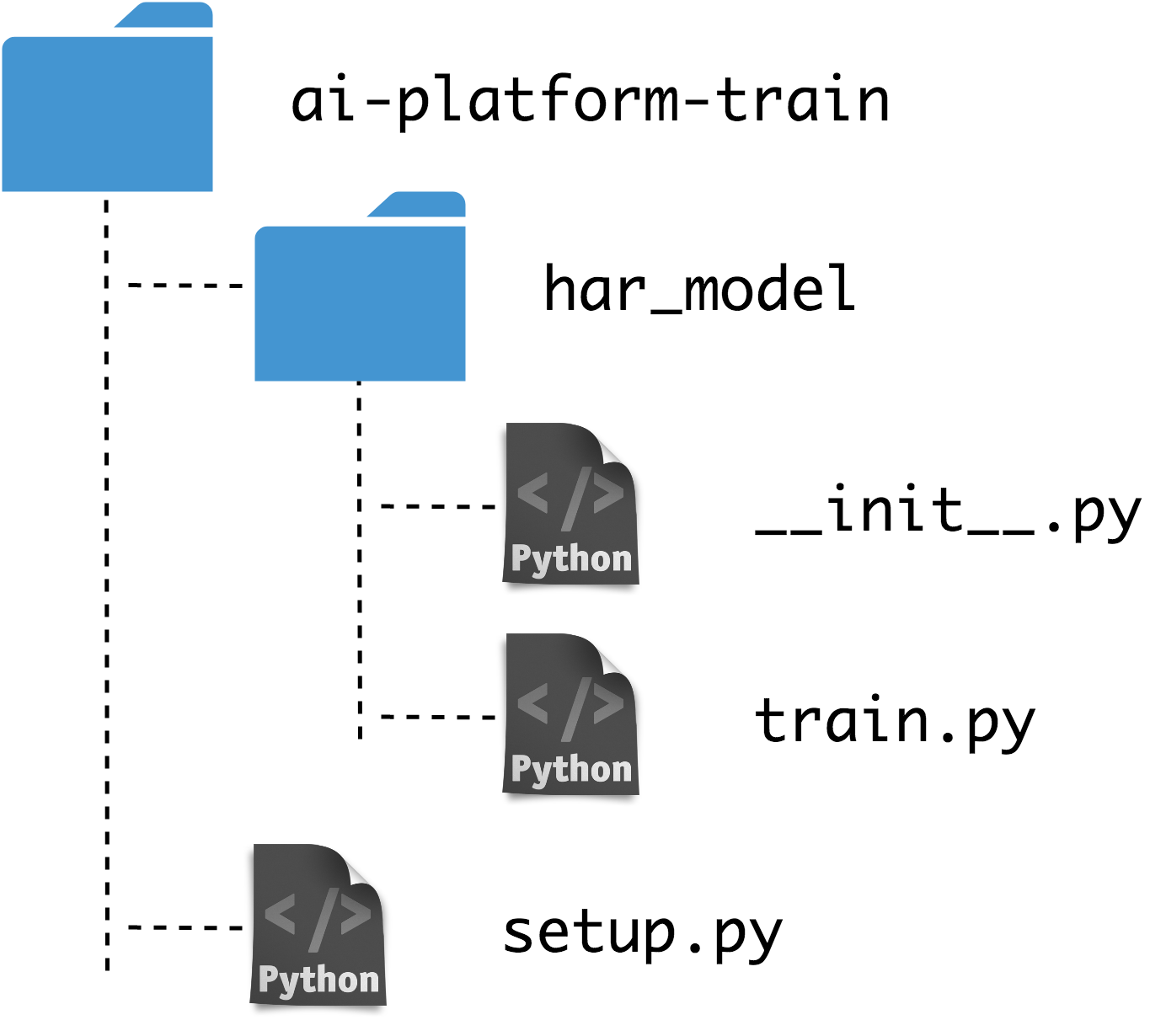Training directory tree

Note that we are also including an empty "__init__.py" so that Python treats the "har_model" directory as a package. The "setup.py" script installs the package along with the required dependencies:

from setuptools import setup, find_packages


DEPENDENCIES = ['vaex-core==4.1.0',
                'vaex-hdf5==0.7.0',
                'vaex-ml==0.11.1',
                'lightgbm==3.1.1',
                'cloudpickle==1.6.0',
                'gcsfs==0.7.1',
                'astropy==4.1']

setup(name='har_model',
      install_requires=DEPENDENCIES,
      include_package_date=True,
      packages=find_packages(),
      description='Create a Human Activity Recognition model from accelerometer data.')

The nice thing about the AI Platform is that we can run our package locally before submitting a job to the GCP. This is quite useful for debugging and testing purposes. The following shell command will execute the training script locally, in the same manner as in the cloud:

gcloud ai-platform local train \
    --package-path="./har_model/" \
    --module-name="har_model.train"

Since the core technology in the current solution is Vaex, one can quite easily limit it to use a small fraction of the data to make the tests run faster. Once we are sure that the training module works as expected, we can submit the training job to GCP via the following command:

gcloud ai-platform jobs submit training $JOB_NAME \
    --job-dir=gs://vaex-data/models \
    --package-path=./har_model/ \
    --module-name=har_model.train \
    --region=europe-west4 \
    --runtime-version=2.3 \
    --python-version=3.7 \
    --scale-tier=CUSTOM \
    --master-machine-type=n1-highcpu-32

Given the large number of parameters, it can be rather convenient to execute the above command as a part of a shell script. That way, it can be version controlled, or part of a CI/CD pipeline for example.

Once the above command is executed, the AI Platform training job will start and you can monitor its progress in the Logging section of GCP. With the machine type we choose in the above example (n1-highcpu-32, 32vCPUs, 28GB RAM), the entire training job takes ~20 minutes. Once the job is finished, we can examine the logs to see how model has done on the test set:

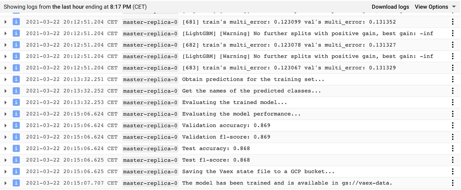Screenshot of the GCP Log Viewer showing the log output of the training job described in the text above.

That is it - with a minimal set up we successfully trained a fully custom Vaex pipeline on GCP! The pipeline itself, which contains the full feature engineering & data processing steps, the classification algorithm and the post processing manipulations, has the form of a Vaex state file and is saved to the designated GCS bucket, ready to be deployed.

Deploying a Vaex pipeline on GCP

The AI Platform is a rather convenient way to deploy ML models. It ensures high availability of the prediction service, and makes it easy to deploy and query multiple model versions, which is useful for doing A/B testing for example.

Deploying a Vaex pipeline is quite simple - all a prediction server needs to do, is to convert the incoming batches or data samples to a Vaex DataFrame, and apply the state file to it. 

In order to deploy a custom Vaex pipeline, we must instruct the AI Platform on how to handle the requests that are specific to our problem. We can do this by writing a small class which implements the Predictor interface:

class VaexPredictor():
    def __init__(self, state=None):
        self.state = state

    def predict(self, instances, **kwargs):

        if isinstance(instances[0], list):
            data = np.asarray(instances).T
            df = vaex.from_arrays(Arrival_Time=data[0],
                                  Creation_Time=data[1],
                                  x=data[2],
                                  y=data[3],
                                  z=data[4])

        elif isinstance(instances[0], dict):
            dfs = []
            for instance in instances:
                df = vaex.from_dict(instance)
                dfs.append(df)
            df = vaex.concat(dfs)

        else:
            return ['invalid input format']

        df.state_set(self.state, set_filter=False)
        return df.pred_name.tolist()

    @classmethod
    def from_path(cls, model_dir):
        model_path = os.path.join(model_dir, 'state.json')
        with open(model_path) as f:
            state = json.load(f)

        return cls(state)

The above VaexPredictor class has two key methods: the from_path method simply reads the state file from a GCS bucket, while the predict method converts the data to a Vaex DataFrame format, applies the state file to it, and returns the predictions. Notice that the predict method conveniently intercepts data that has been passed either as a Python list or dict type.

The next step is to package the VaexPredictor class as a .tar.gz source distribution Python package. The package needs to include all the dependencies that are needed for obtaining the predictions. Creating such a package needs a "setup.py" file:

import os
from setuptools import setup, find_packages


os.environ['HOME'] = '/tmp'

DEPENDENCIES = ['vaex-core==4.1.0',
                'vaex-ml==0.11.1',
                'lightgbm==3.1.1',
                'cloudpickle==1.6.0',
                'gcsfs==0.7.1',
                'astropy==4.1']

setup(
    name='vaex_predictor',
    scripts=['predictor.py'],
    install_requires=DEPENDENCIES,
    include_package_date=True,
    packages=find_packages(),
    description='Prediction routine for the Human Activity Recognition phone accelerometer model.')

The package is created by running the following shell command:

python setup.py sdist --formats=gztar

Finally, we need to move the prediction package to GCS, so the AI Platform can pick it up and deploy it:

gsutil cp dist/vaex_predictor-0.0.0.tar.gz $BUCKET/deployments/

It may come in handy to bundle the above two commands in a bash script for convenience, especially if one needs to iterate a few times while creating the prediction package.

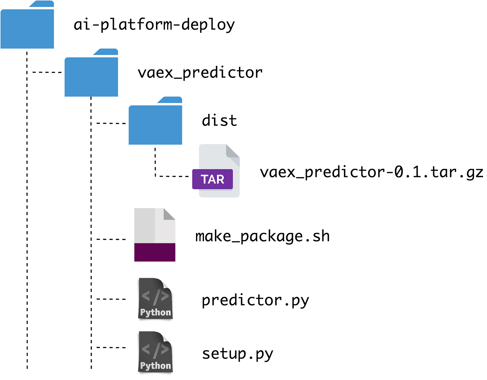
For reference, the directory tree of deployment part of this example project should look something like this:

We are now ready to deploy the prediction package. It can be rather convenient to define some environmental variables in the shell first:

# The model name
MODEL=har

# Version name
VERSION=v1

# The region
REGION=global

# Specify the runtime version. Each version comes pre-installed with specific dependencies.
RUNTIME_VERSION=2.3

# Which python version to run
PYTHON_VERSION=3.7

# Path to the directory containing the model state file
ORIGIN=gs://vaex-data/models/har_phones_accelerometer_2021-03-22T19:15:06

# Path to prediction module
PREDICTION_PACKAGE_PATH=gs://vaex-data/deployments/vaex_predictor-0.0.0.tar.gz

# The prediction class, located within the prediction module
PREDICTION_CLASS=predictor.VaexPredictor

The model deployment is done with the following two commands. First we need to create a "model" resource on the AI Platform like so:

gcloud beta ai-platform models create $MODEL \
  --region=$REGION \
  --enable-logging \
  --enable-console-logging

Then we create a "version" resource of the model, which points to the model artefact, i.e. the state file, and the predictor class:

gcloud beta ai-platform versions create $VERSION \
    --model=$MODEL \
    --region=$REGION \
    --runtime-version=$RUNTIME_VERSION \
    --python-version=$PYTHON_VERSION \
    --origin=$ORIGIN \
    --package-uris=$PREDICTION_PACKAGE_PATH \
    --prediction-class=$PREDICTION_CLASS

It may take a minute or two before the above command executes. That's it! Our Vaex model is now deployed and is ready to respond to incoming prediction requests!

We are now ready to query our model. The batches of data sent to the AI Platform need to be in a JSON format. If the input has the form of lists, each row of the file should be a list containing the features of a single sample. Care should be taken that the order of features are consistent with what is expected by the Predictor class. And example of such a file is shown below:

[1424697931391,275463508651000,-4.913,-2.413,9.692]
[1424787692560,13362572400000,3.677,-0.306,9.5]
[1424782921581,8591592450000,-3.065,-2.298,12.105]
[1424787476448,1424787479929268498,-2.732,-0.151,9.946]
[1424785658500,8908695829000,-0.233,1.123,7.609]
[1424697078597,1424698924651879163,0.255,-0.679,9.813]
[1424782108573,5874182665000,3.15,0.47,8.896]
[1424781121454,5035895191000,-1.827,3.03,8.425]
[1424695080663,1424696926717728579,-11.444,6.331,12.429]

Prediction requests are then sent with the following command:

gcloud ai-platform predict --model=$MODEL --version=$VERSION --json-instances=input_list.json --region=$REGION

The input data can also be formatted as JSON objects. One can be more flexible here - one line can be a single or multiple samples:

{"Arrival_Time": [1424697931391, 1424787692560, 1424782921581],
 "Creation_Time": [275463508651000, 13362572400000, 8591592450000],
 "x": [ -4.912, 3.677, -3.064],
 "y": [-2.413, -0.301, -2.298],
 "z": [ 9.692,  9.501, 12.104]}
{"Arrival_Time": [1424787476448, 1424785658500, 1424697078597],
 "Creation_Time": [1424787479929268498, 8908695829000, 1424698924651879163],
 "x": [-2.731, -0.233, 0.254],
 "y": [-0.151, 1.122, -0.679],
 "z": [9.941, 7.602, 9.813]}
{"Arrival_Time": [1424782108573, 1424781121454, 1424695080663],
 "Creation_Time": [5874182665000, 5035895191000, 1424696926717728579],
 "x": [3.149, -1.820, -11.400],
 "y": [0.420, 3.029, 6.333],
 "z": [8.895,  8.301, 12.421]}

The following is a short screen cast of querying our "har_model" with the file above:

It is that simple!  The lives of ML models are not infinite. When the time comes to undeploy a model, one needs to first delete the version resource, and then delete the model resource:

# Delete a model version
gcloud ai-platform versions delete $VERSION --model=$MODEL --region=$REGION

# Delete the model
gcloud ai-platform models delete $MODEL --region=$REGION

Finally, it may be important to note that even though we trained the model on GCP in this example, this is not at all a deployment requirement. All that is required is for the state file to reside in a GCS bucket, so that the prediction module can pick it up. One can train the model and create the state file locally, or using any other service that is available out there.

Summary

I hope this article demonstrated that Vaex is an excellent tool for building ML solutions. It's expression system and automatic pipelines are especially useful for this task, while its efficient, out-of-core algorithms ensure speed and keeps computational costs low. 

Using Vaex in combination with GCP brings considerable value. Vaex is able to stream data directly from GCS, and only those portions that are absolutely necessary to the model. Training ML models on Google Clouds' AI Platform is also rather convenient, especially for the more demanding, longer running models. Since the entire transformation pipeline of a Vaex model is contained within a single state file, deploying it with the AI Platform is straightforward. 

Happy data sciencing!

Appendix: AI Platform Unified

In mid-November 2020 Google launched the next iteration of the AI Platform, dubbed AI Platform Unified. As the name suggest, this version unifies all ML related services that GCP offers: autoML, ready to use APIs as well as options to train and deploy custom models can all be found in the same place. 

One significant improvement that the new AI Platform brings is the option to train and deploy models using custom Docker containers. This brings additional flexibility compared to the "classical" AI Platform in which only specific environments are available with a limited options to install or modify their contents.

Lets see how we can use the Unified AI Platform to train and deploy the Vaex solution we built earlier in this article, now using custom Docker containers. 

Training the model is rather straightforward: all we need to do is create a Docker image that when started will execute the training script we prepared earlier. We begin by creating a Dockerfile:

FROM condaforge/mambaforge:4.9.2-5 as conda

# Copy relevant files & config & training package
COPY env.yml setup.py ./
ADD har_model ./har_model/

# Create the environment and install the training package
RUN mamba env create -f env.yml
RUN echo "source activate training-image" > ~/.bashrc \
    && conda clean --all --yes
ENV PATH /opt/conda/envs/training-image/bin:$PATH
RUN pip install -e .

# Run the container
ENTRYPOINT ["python", "har_model/train.py"]

In the above Dockerfile, "env.yml" all the dependencies we need that can be install via either conda, mamba, or pip. The "setup.py" and "har_model" make up the model training package we defined earlier. We then install the required dependencies and the model training package, and finally set up an entrypoint so that the training process starts when the container is run. Pro-tip: if you want to build very small Docker containers check out this guide by Uwe Korn.

Now, we can build the Docker image locally and push it to Google's Container Registry, but it is much more convenient to simply use Cloud Build and build the image right in GCP:

gcloud builds submit --tag $CUSTOM_CONTAINER_IMAGE_URI

Then we can launch the container and start the training job simply by executing:

gcloud beta ai custom-jobs create \
  --region=$REGION \
  --display-name=$JOB_NAME \
  --worker-pool-spec=machine-type=$MASTER_MACHINE_TYPE,replica-count=1,container-image-uri=$CUSTOM_CONTAINER_IMAGE_URI

The training progress can be monitored via Cloud Logging, which captures any logs that come out of the custom Docker container. Some 20 minutes later the job should finish, and we can inspect it via the Google Cloud Console:

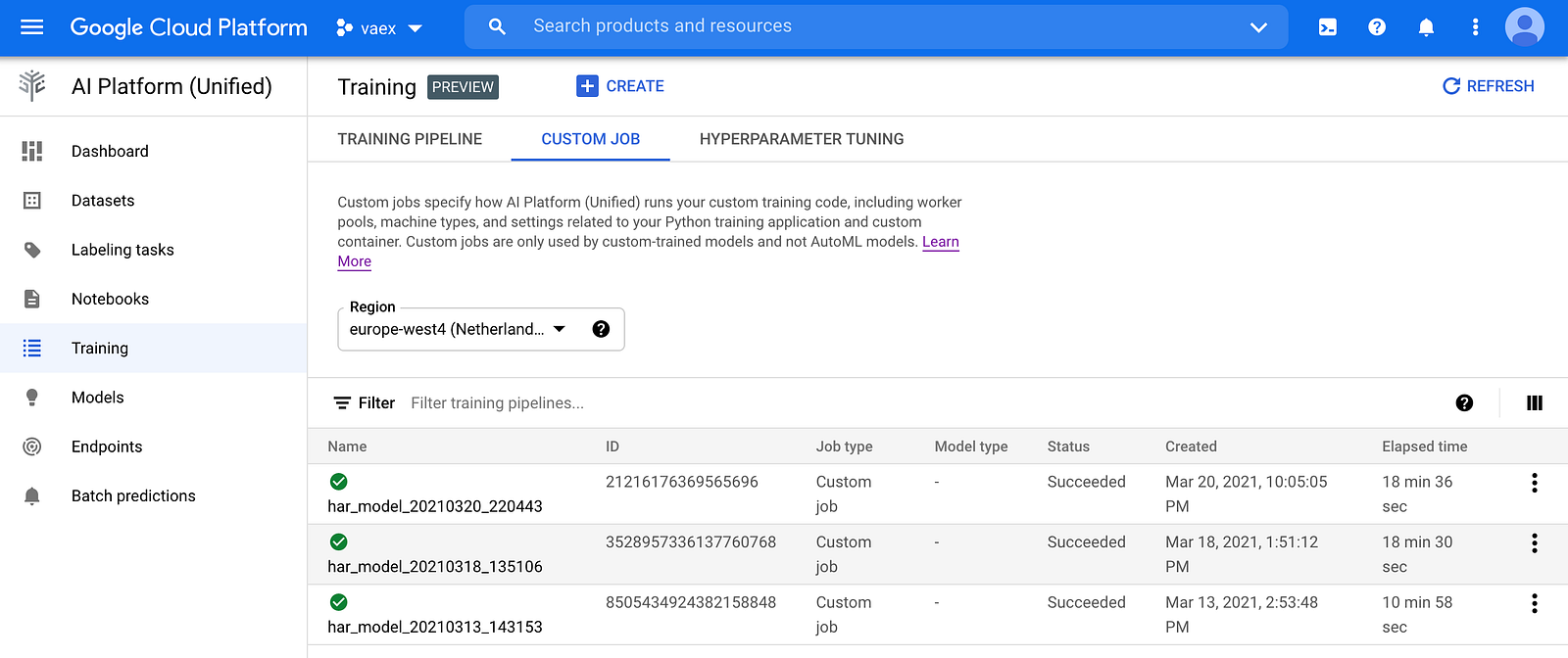
Now let us deploy the model we just trained using a custom Docker container on the Unified AI Platform. When started, the container should run a web application that will respond to requests with the predictions. The web application should implement at least two method: one that the AI Platform will use to make "health checks" i.e. make sure the web application is running as expected, and another method which will accept incoming prediction requests and respond with the answers. For more information on the requirements of the container and all available options for customization you can check out the official documentation.

We will not go into detail in how to build such a web application, as there are plenty of resources on the web focusing on this. For reference, you can see the web application we have prepared for this example here.

After building and testing the web application, we need to create a Docker container that will run it when started. This is easily done following the same steps for creating the model training container. 

Once the Docker image is available in Container Registry, we need to make a model resource out of it via the following gcloud command:

gcloud beta ai models upload \
  --region=$REGION \
  --display-name=$MODEL_NAME \
  --container-image-uri=$CUSTOM_CONTAINER_IMAGE_URI \
  --artifact-uri=$PATH_TO_STATE_FILE \
  --container-health-route=/health \
  --container-ports=8000 \
  --container-predict-route=/predict

The next step is to create a model endpoint used to access the model:

gcloud beta ai endpoints create \
  --region=$REGION \
  --display-name=$ENDPOINT_NAME

We can now deploy the model resource to the endpoint like this:

gcloud beta ai endpoints deploy-model $ENDPOINT_ID \
  --region=$REGION \
  --model=$MODEL_ID \
  --display-name=deployed_har_model \
  --machine-type=n1-standard-2 \
  --min-replica-count=1 \
  --max-replica-count=1 \
  --traffic-split=0=100 \
  --enable-access-logging \
  --enable-container-logging

This step may take a few minutes to complete. Note that you can deploy several model resources to a single endpoint, as well as have a single model deployed to multiple endpoints. 

The model now is finally deployed and ready to accept requests. The requests should be in JSON format and have the following structure:

{
    "instances":[
        {"feature_1": [1, 2, 3],
         "feature_2": [10, 20, 30],
         "feature_3": ["a", "b", "c"]},
        {"feature_1": [4, 5, 6],
         "feature_2": [40, 50, 60],
         "feature_3": ["e", "f", "g"]}
    ],
    "parameters": {"param1": "value1", "param2": "value2"}
}

Here you see how such a file would look like for this particular example. The Google Cloud Console will also give you an example of how to query the model endpoint. It will look something like this:

That's it! When your model outlives its lifetime, do not forget to undeploy it and delete the endpoint and model resource, as to avoid unwanted costs. That can be done like this:

# Undeploy the model
gcloud beta ai endpoints undeploy-model $ENDPOINT_ID \
  --project=$PROJECTID  \
  --region=$REGION \
  --deployed-model-id=$DEPLOYED_MODEL_ID

# Delete the endpoint
gcloud beta ai endpoints delete $ENDPOINT_ID --region=$REGION

# Delete the model resource
gcloud beta ai models delete $MODEL_ID --region=$REGION

As a final note, one can think of training and deployment as two separate, fully independent processes. This means that one can use the "classical" AI Platform to train, and the Unified AI Platform to deploy the model, and vice-versa. Of course, one can always create the model "in house" or using any resources available out there, and just use GCP for serving.