“Data is the new oil.” Regardless of whether or not you agree with this statement, the race for gathering and exploiting data has been going on for a while now. In fact, one thing the tech giants of today have in common, is their capacity to fully exploit the enormous quantity of data they gather. They have the knowledge, manpower, and resources to analyse billions of data points, train and deploy a variety of machine learning models at scale, which then impacts countless people across our planet.

Creating even a simple machine learning service is a non-trivial task. Even if we ignore the data gathering and augmentation steps, one still needs to understand the data, clean it appropriately, create meaningful features, and then train and tune a model. This is followed by a series of validation steps which hopefully lead to a better understanding of both the data and the model. The process is repeated until the model satisfies the business goals, after which it is put in production. In practice, however, the process may continue indefinitely.

Imagine that we have a dataset containing over 1 billion samples, which we need to use for training of a machine learning model. Due to the sheer amount alone, exploring such dataset already becomes tricky, while iterating on the cleaning, pre-processing and training steps becomes a daunting task. Challenges such as these are commonly tackled with distributed or cloud computing. While this is the standard approach today, it can be quite costly, time-consuming, and simply less convenient compared to working on your local machine.

In this article, I will demonstrate how anyone can train a machine learning model on a billion samples in a swift and efficient manner. Your laptop is all the infrastructure you need. Just make sure it is plugged in.

The problem: predict taxi trip duration

As an example, assume we would like to help a taxi company predict how long a trip may take in New York City. We will use the New York City Taxi dataset, which contains information on over 1 billion taxi trips conducted between 2009 and 2015 by the recognizable Yellow Taxis. In its raw form, the data is provided by the New York City Taxi & Limousine Commission (TLC), and can be downloaded from their website. If you are simply interested in the Jupyter notebook used as the basis for this article, you can click here.

Data preparation with Vaex

In order to manipulate the large amount of data, we will use Vaex, a Python open-source DataFrame library. Leveraging concepts like memory mapping, lazy evaluations and efficient out-of-core algorithms, Vaex can easily handle datasets that would otherwise be too large to fit in RAM.

Let’s get started by opening the data. For convenience, I’ve combined the 7 year of taxi data into a single HDF5 file. Even though the file is larger than 100GB on disk, opening it with Vaex is instantaneous:

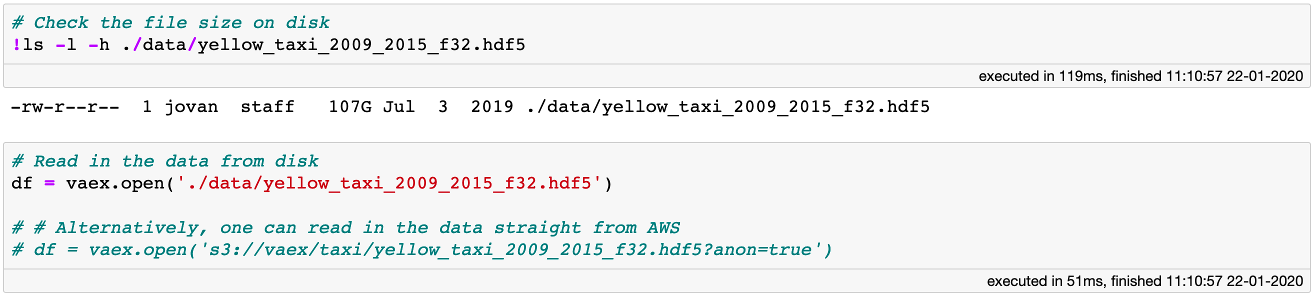Opening an memory-mapped file is instant (119 ms!) with Vaex. If you don’t have it locally, you can lazily stream it from AWS.

Inspecting the data is just as fast. Since the data is memory-mapped, Vaex knows immediately where to look, reading only the portions that are needed. For a simple preview as shown below, only the first and last 5 rows are read from disk.

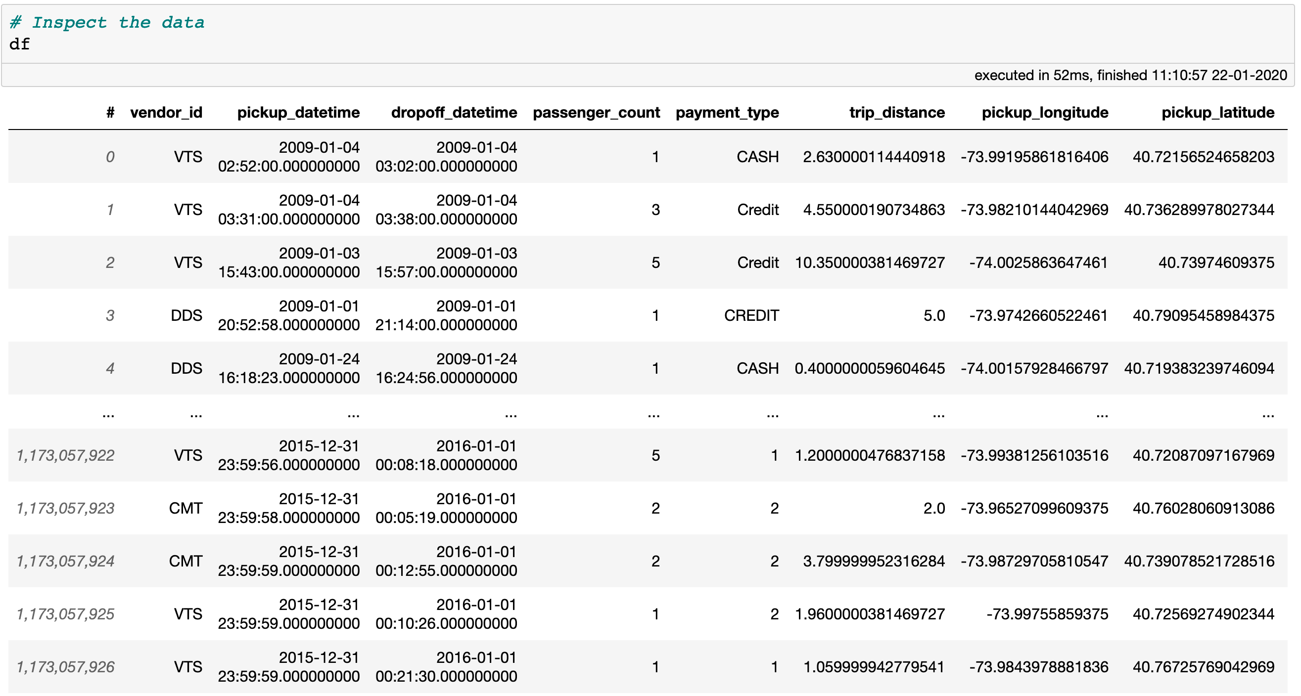A preview of the Taxi Dataset. Only the first and last 5 rows are actually read from disk.

Working with the New York Taxi dataset is rather straightforward with Vaex, despite being over 100GB on disk and containing more than 1.1 billion records. This article goes over the Vaex fundamentals, and presents an exploratory data analysis of this very same dataset.

Before we get started, let us split the data into a train and a test set. We will make the split by year, such that the trips conducted in 2015 will comprise the test set, and all prior to that will make up the training set. The dataset is ordered by year, so we can do the splitting by simply slicing the DataFrame.

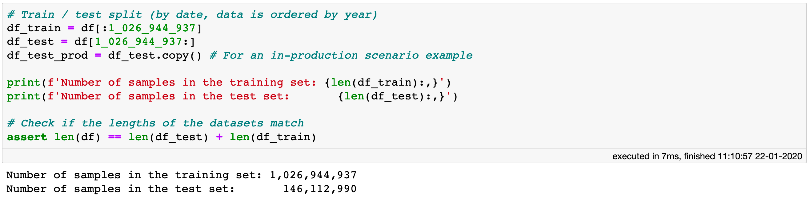Create train and test sets. Slicing of a Vaex DataFrame does not copy the data, but only creates a reference.

Note that no memory copies of the data are made by executing the above code cell. Slicing a Vaex DataFrame results in a shallow copy, which only references the appropriate portions of the original data.

Data wrangling

The goal of this exercise is to predict the likely duration of a taxi trip. The duration of a trip is not readily available in the dataset, but it is trivial to calculate from the pick-up and drop-off time-stamps.

Creating a new column out of existing columns costs no extra memory, and is instant.

Calculating the trip distance in the code example above results in a virtual column. Creating such columns cost no memory, since they store just the expression that defines them, and are evaluated only when necessary.

Now, let’s filter out outliers and erroneous data samples from the training set. The exploratory data analysis presented in this article can serve as a guide on how to do this, so please check it out of if you would like to know the rationale behind these filtering choices.

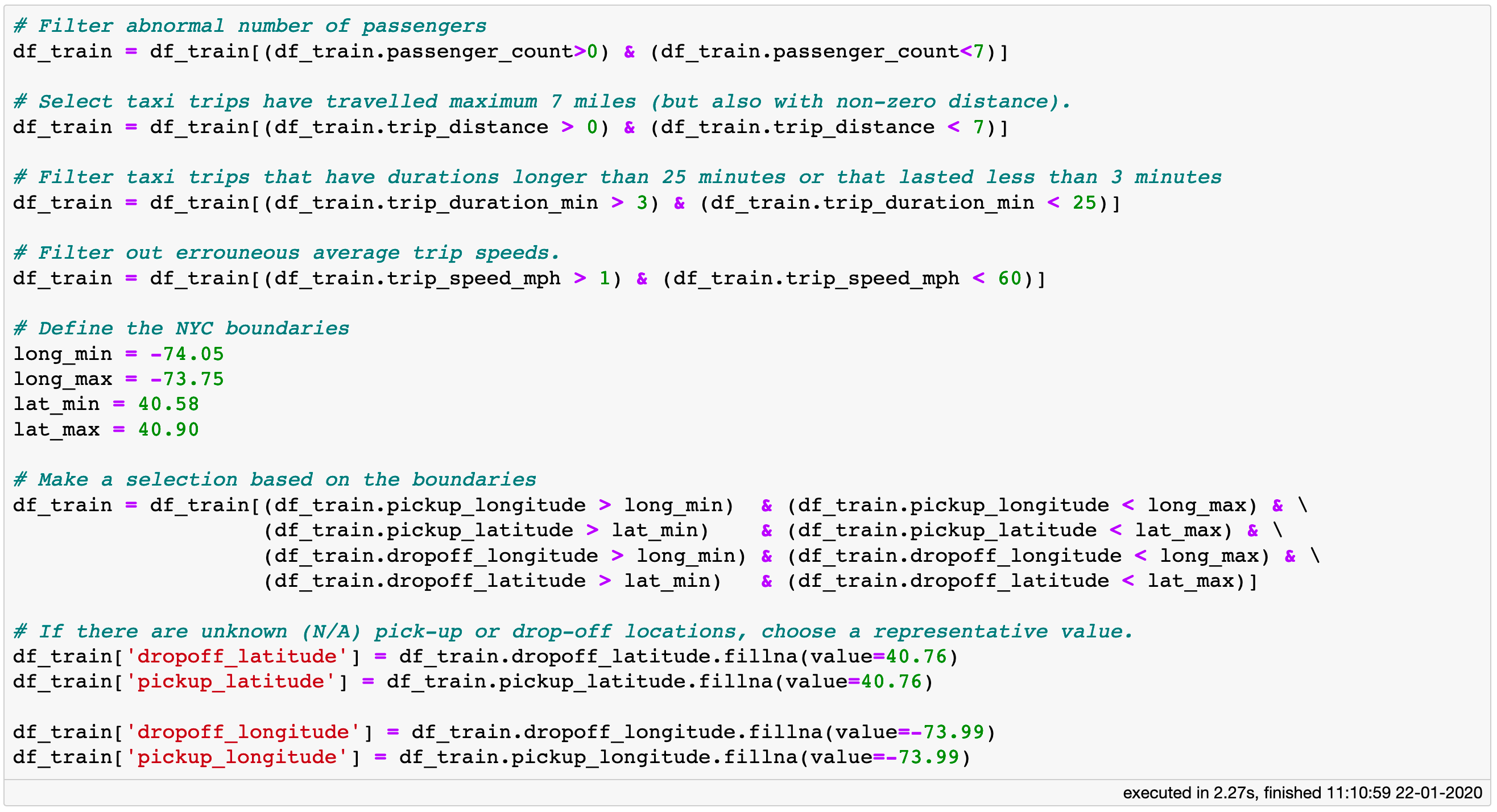Filtering out a Vaex DataFrame takes seconds and costs no extra memory, even when it numbers billion rows.

The main idea behind the filtering is to remove outliers and possible erroneous data inputs, so the model is not too “distracted” by the few abnormal samples. After all the filters are applied, the training set comprises “only” 812,816,595 taxi trips.

At this stage we can start to engineer some meaningful features. Since all of the features we will be virtual columns, we do not need to concern ourselves with memory usage, and thus have the freedom to experiment and get creative. Let’s begin by extracting few features from the pick-up timestamps.

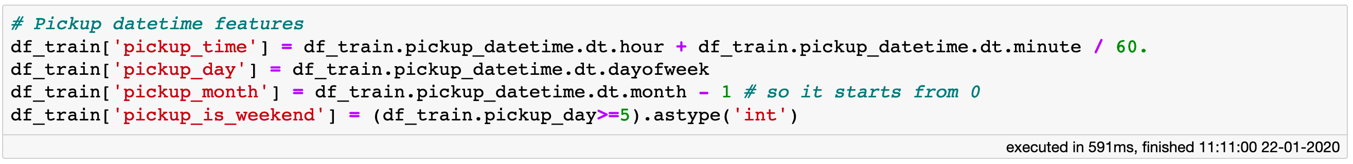Extracting some useful features from the pick-up date and time.

Now, let us create a couple of more computationally demanding features. One of them is the distance between the pick-up and drop-off points, which we will call the “arc distance”. The second feature is the direction angle of the taxi trip, i.e. an indication of whether the taxi is travelling for example due north or north-west from its origin towards its destination.

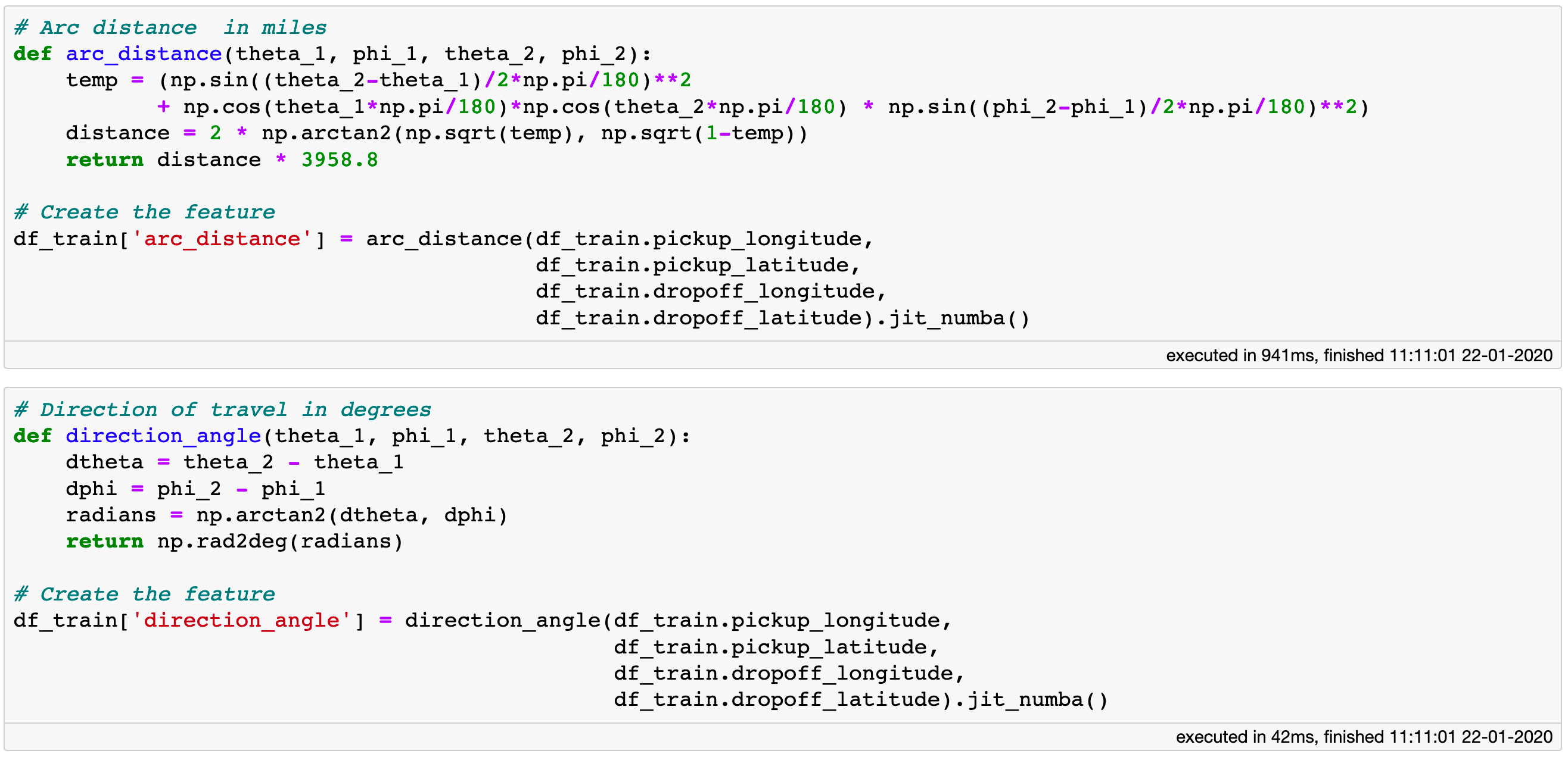The evaluation of computationally demanding expressions can be sped up by Just-In-Time compilation via Numba or CUDA.

Notice the .jit_numba method at the end of the function call. The evaluation of computationally expensive expressions like those defined above can be accelerated by Just-In-Time compilation via Numba. If your machine sports a more recent NVIDIA graphics card, you can use CUDA by invoking the .jit_cuda method for an extra boost. By using .jit_numba on some expressions and .jit_cuda on others, you can simultaneously leverage both your CPU and GPU for maximum performance.

Data transformation (vaex.ml)

Before we pass the data to any model, we need to make sure it is suitably transformed in order to get the most out of it. Vaex contains the vaex.ml package which implements a variety of common data transformations, such as PCA, categorical encoders, and numerical scalers. All transformations are invoked with the familiar scikit-learn API, are parallelised and executed out-of-core.

Let’s focus on the pick-up and drop-off locations. In many cities in the United States the streets form a grid pattern. This is clearly visible in the Manhattan area. One idea to improve the performance of a model is to apply a set of PCA transformations on the pick-up and drop-off locations. This will cause the streets, traced by the many pick-up and drop-off points, to align with the natural geographical axes (longitude and latitude) instead of being at an angle to them.

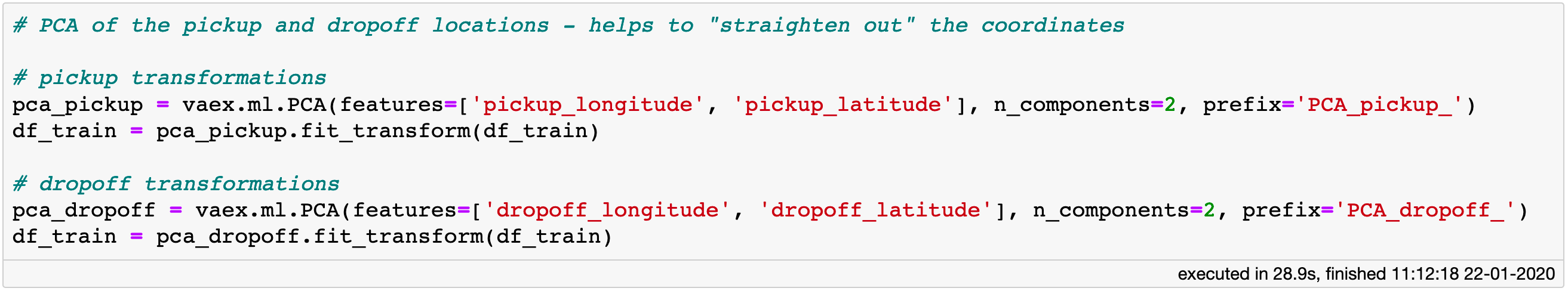Fitting a couple of PCA transformers on nearly billion samples takes about half a minute with vaex.ml.

Notice that when using vaex.ml one passes the whole DataFrame to the .fit, .transform, or .fit_transform methods of a transformer, while the features on which the transformation is applied are specified while that transformer is instantiated. Most importantly, the .transform method returns a shallow copy of the DataFrame in which the result of the transformation is stored in the form of virtual columns. This makes it easy for us to visualise the results of the PCA transformations.

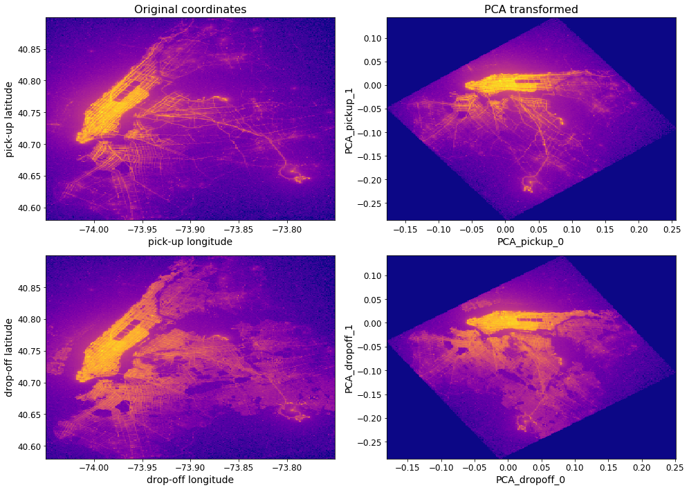Comparing the original to the PCA-transformed pick-up and drop-off locations.

Let us shift our focus on the “pickup_time”, “pickup_day” , and “pickup_month” features we defined earlier. The key property of these features is that they are cyclical in nature, i.e. January is as close to February as it is close to December. Thus we will use the CycleTransformer implemented in vaex.ml which essentially treats each feature as the angle φ in a unit circle in polar coordinates (ρ=1, φ). The, transformer than computes the 𝑥 and 𝑦 projection of the radius ρ, thus getting two new components per feature. This trick perfectly preserves the relative distance between different values, since it is simply a coordinate transformation. You can read more about this approach in this post.

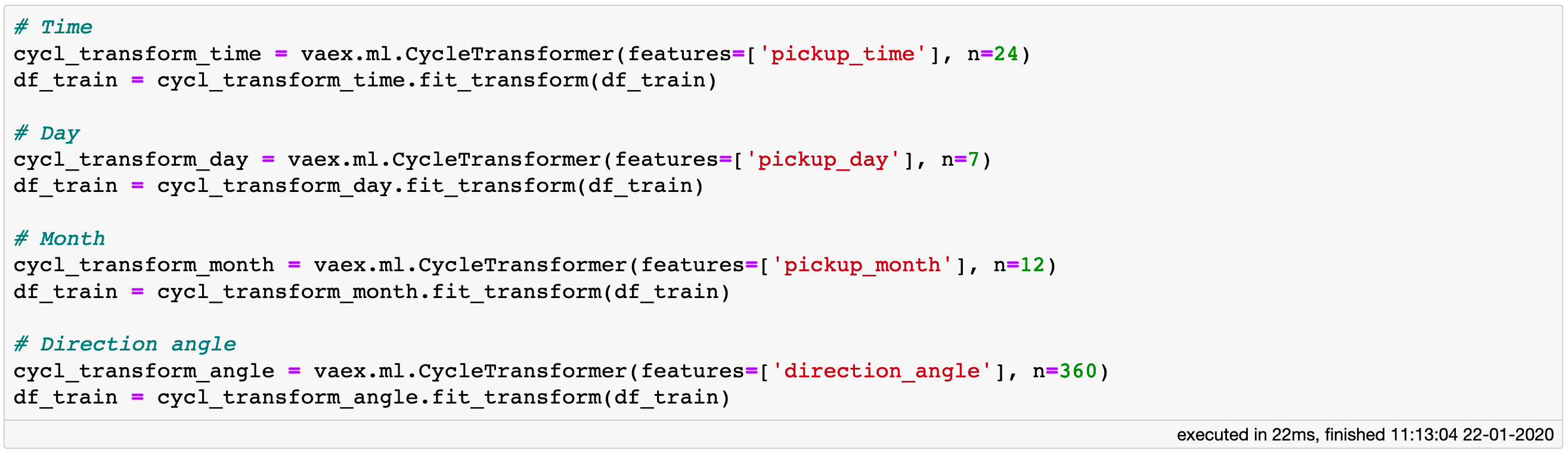Encoding the cyclical features with vaex.ml.CycleTransformer perfectly preserves the relative distance between different values.

We apply the same trick to the direction angle, since it is a cyclical feature as well. Let’s plot the features derived from the “pickup_time” column, as to convince ourselves that the transformations make sense.

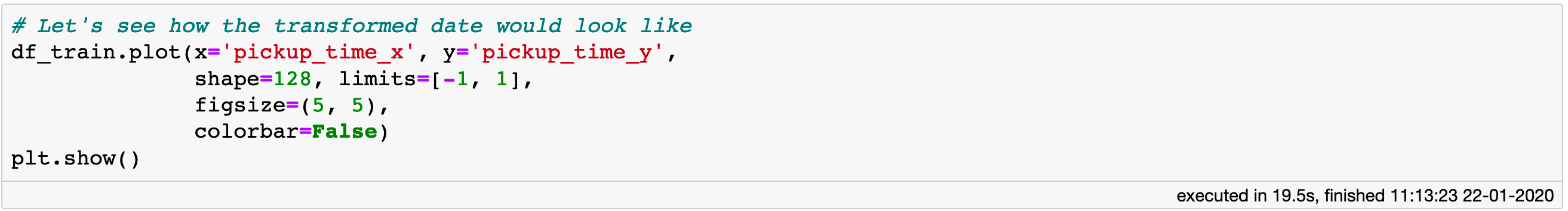
*Density map of the *𝑥 and 𝑦 projections of the “pickup_time” feature.

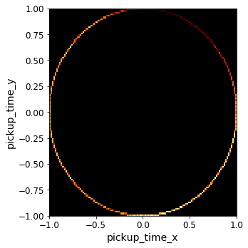
We see that the transformed features create a perfect unit circle. Note that, unlike a regular wall clock, all 24 hours are represented on the circle. For example, “midnight” has coordinates *(x, y) = (1, 0), *“6 o’clock” is at *(x, y) = (0, 1), *while “noon” is at (x, y) = (-1, 0).

Lastly, we only have one continuous feature, “arc_distance” , which we have not paid any attention to. We are simply going to apply standard scaling to it.

Standard scaling transformation of a continuous feature with vaex.ml.

Now that we are done with all of the pre-processing tasks, we can create a final list of features we are going to use for training the model.

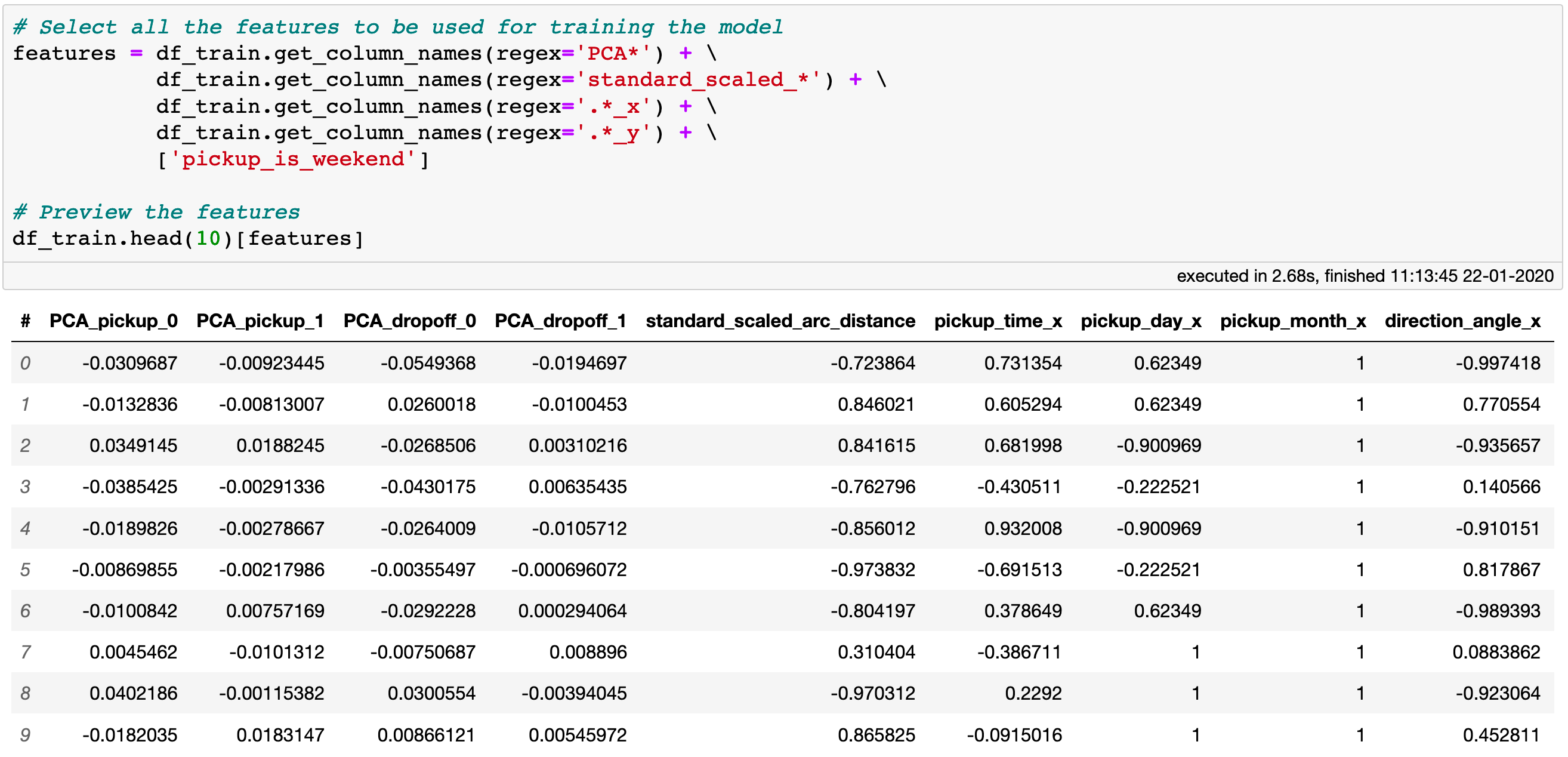A subset of the features used for training the model.

Training the model: Vaex + scikit-learn

At this stage we are ready for the model training phase. While vaex.ml does not yet implement any predictive models, it does provide an interface to several of the popular machine learning libraries in the Python ecosystem such as scikit-learn and xgboost. The benefit of using these models via Vaex is that one does not waste any memory while doing the data cleaning, feature engineering and pre-preprocessing, and thus maximizes the available RAM for training the model.

For the current problem, we are still in need of significantly more RAM than available on a typical laptop or desktop computer if we were to materialize all the features we intend to use for the training. To circumvent this issue, we will make use of the SGDRegressor available via scikit-learn. SGDRegressor belongs to a family of predictive models in scikit-learn that, besides the usual .fit, also implement a .partial_fit method. This allows the model to be trained on batches of data, essentially making it out-of-core.

With the wrapper implemented in vaex.ml one can easily send batches of data from a Vaex DataFrame to the scikit-learn model. The use is straightforward. First instantiate the SGDRegressor from scikit-learn while setting its parameters in the standard way. Then instantiate the IncrementalPredictor implemented in vaex.ml while also providing the main model, a list of features names, the name of the target column, and the batch size. In principle any model can be used as long as it has a .partial_fit method and follows the scikit-learn API convention. Through the batch size one can control the RAM usage. Optionally one can also specify the number of epochs, i.e. how many times the data in each batch is seen by the model, and whether it should be shuffled or not. Finally we call the .fit method on the IncrementalPredictor instance, where we pass the training set DataFrame.

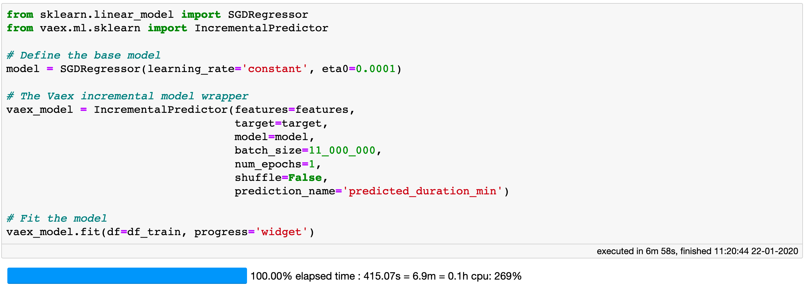Training a model on ~1 billion samples is easy and fast with Vaex and scikit-learn.

It is quite remarkable that this Vaex + scikit-learn combo lead to a total training time of just 7 minutes on my laptop (MacBook Pro 15", 2018, 2.6GHz Intel Core i7, 32GB RAM). This includes on-the-fly evaluation of the 14 features used, all of which are virtual columns, and training the scikit-learn model. In addition, with the set of parameters shown above, the RAM usage never surpassed 4 GB, which leaves me plenty of room to run Slack.

The exact same setup as shown above was also run by Maarten Breddels on his Lenovo Thinkpad X1 Extreme laptop (Intel Core i7–8750H, 32GB RAM), and the training phase took less than 5 minutes!

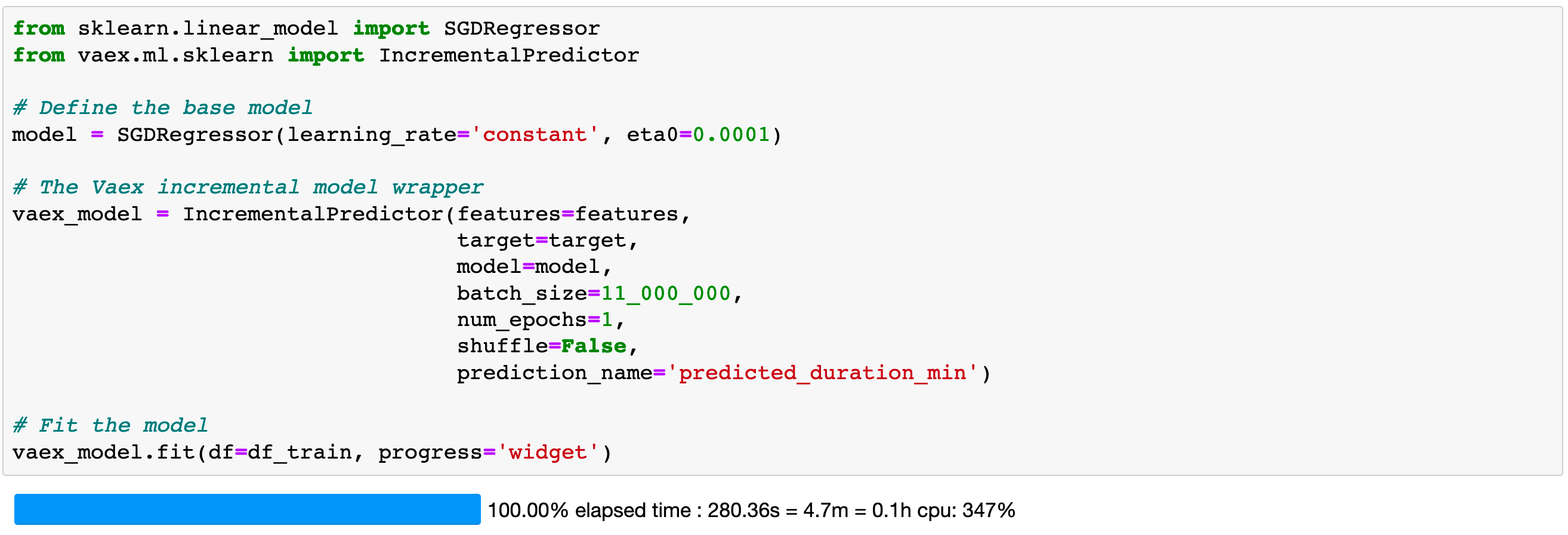Training the SGDRegressor took less than 5 minutes on a Lenovo Thinkpad X1 Extreme laptop (Intel Core i7–8750H, 32GB RAM) running Linux.

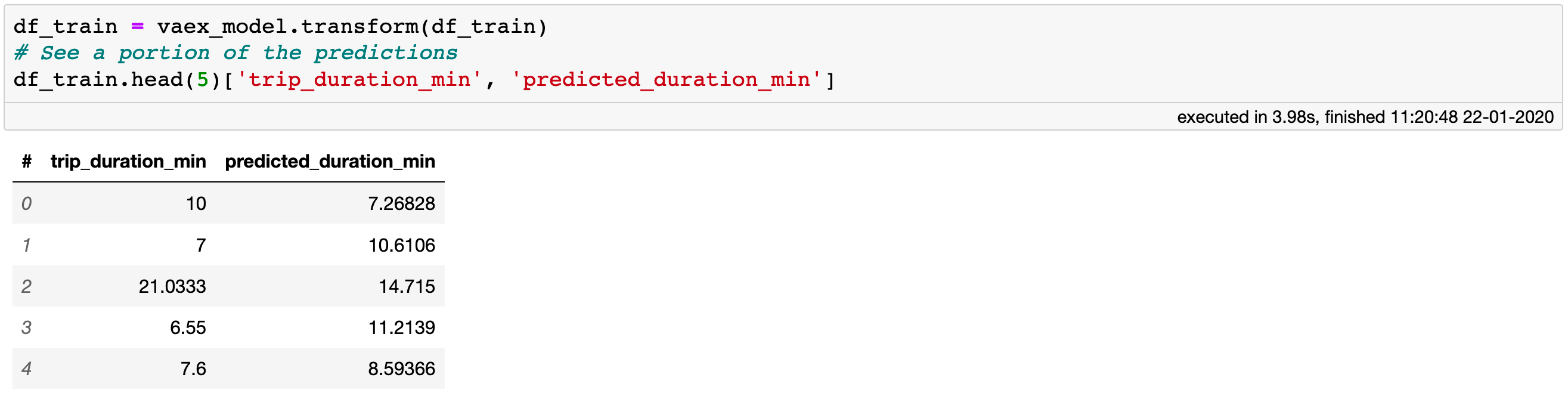
The IncrementalPredictor is not just a convenience class for passing Vaex DataFrames to scikit-learn models. It is also a vaex.ml transformer, meaning that the .transform method returns a shallow copy of a DataFrame containing the model predictions as a virtual column. This is the case for any model wrapper implemented in vaex.ml. Not only does this cost no extra memory, but it also makes it quite convenient to post-process the result and even make ensembles, as well as to calculate various performance metrics and diagnostic plots, as we shall see in a moment.

All model wrappers in vaex.ml are transformers.

Finally, let us constrain the predictions to be within the bounds of the data the model was trained on. This is done to prevent the estimation of unphysical or unrealistic durations for some exotic combinations of feature values. Thus, let us set any predictions smaller than 3 minutes to 3, and any predictions larger than 25 minutes to 25.

The output of a vaex.ml model wrapper is a virtual column, which makes it easy to post-process, or to use for creating diagnostic plots or compute metrics.

What about a pipeline?

Now that the model is trained, we would like to know how well it is doing by applying it on the test set. You may have noticed that, unlike other libraries, we did not explicitly create a pipeline to propagate all the data cleaning and transformation steps. In fact, with Vaex, a pipeline is automatically being created as one is doing exploration and transformation of the data. Each Vaex DataFrame contains a state, which is a serialisable object containing all of the transformations applied to it: filtering, creating new virtual columns, column transformation).

Recall that all of the features we created, along with the output of the PCA transformations, scaling and the predictive model output, including the final tinkering with the predictions are virtual columns, and thus are stored in the state of the training DataFrame. Thus, to calculate the predictions on the test set, all we need to do is to apply this state to that test set DataFrame, and all of the transformations will be automatically propagated.

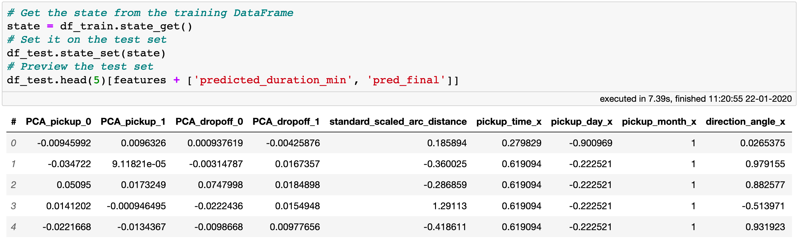Applying the state from the training to the test set results in automatic propagation of filters and virtual columns.

The state can be also serialized and read from disk, which greatly simplifies the task of model deployment.

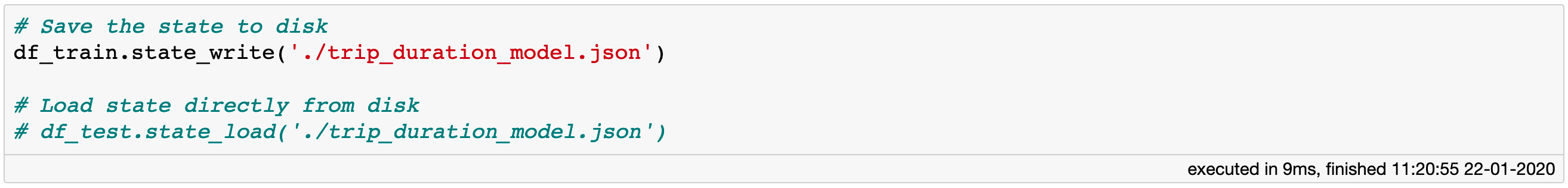The state of a Vaex DataFrame can be easily serialized and read from disk. This is can be extremely useful when deploying the model.

Model diagnostics

Now that the trip duration predictions are available for both the training and the test set, let us calculate some performance metrics. Since this is a regression problem, we will calculate the mean absolute and the mean squared errors.

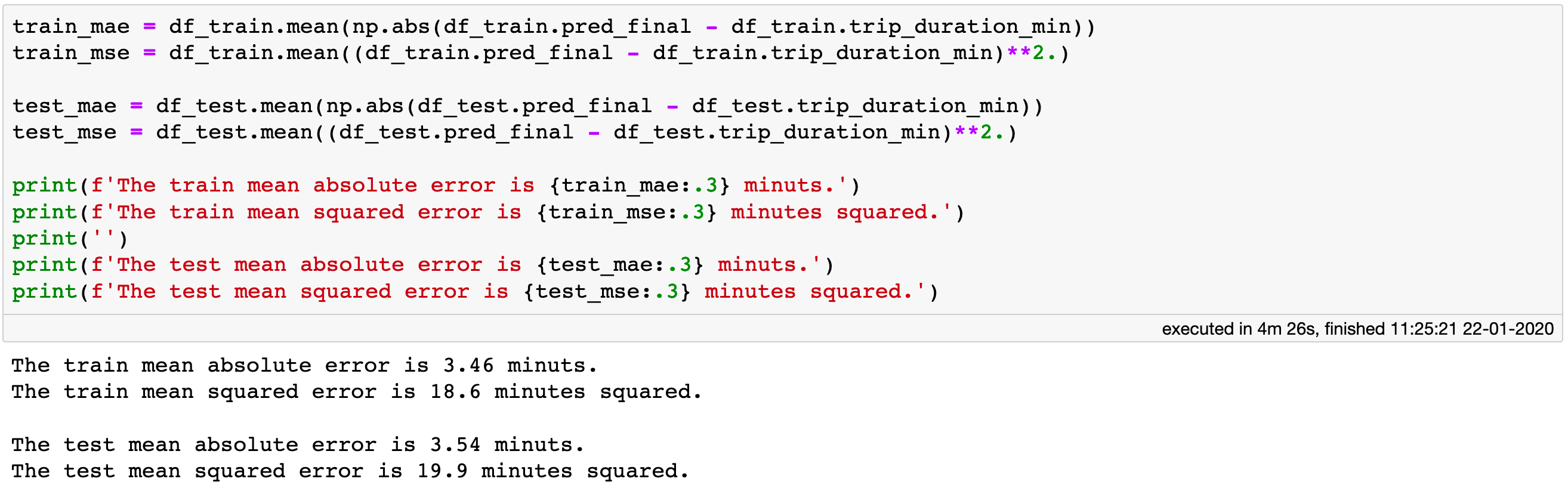Computing the absolute and mean square errors for both the train and the test sets.

Notice that calculation of the 4 statistics shown in the figure above took ~4.5 minutes. This is quite impressive considering that the computation requires evaluating all the features which were then passed on to the model to obtain the predictions, and this was done for over 1 billion samples between the train and the test sets, twice over.

The mean absolute error evaluated on the test set is just over 3.5 minutes. Whether this is an acceptable error, one should probably consult with a frequent taxi passenger or a taxi driver in New York City. We should not accept such statistics at face value, and hence let us create a couple of diagnostic plots. Let us plot the distribution of the actual vs the estimated trip durations, as well as the absolute error of the predicted durations.

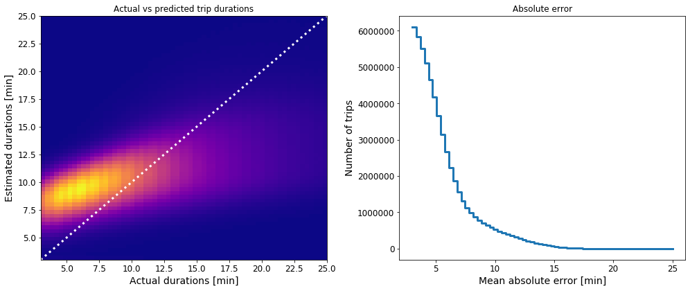Left: A density map of the actual vs the estimated trip durations of the test set. Right: Absolute error of the predicted durations of the test set.

While we see a strong correlation between the actual and the estimated trip durations, the left panel of the figure above also shows that the model estimates are systematically biased to higher values. One potential reason for this is the non-Gaussian distribution of the training features and the target variable. There could also be some outliers that negatively affect the model performance, despite or filtering efforts earlier. On the other hand, it is not that bad to be a bit pessimistic when it comes to estimating taxi trip durations, perhaps.

The right panel shows the number of trips per absolute error bin. In fact, 77% of all trip durations in the test set were estimated with an absolute error of less than 5 minutes. While the current model may serve as a good starting baseline, there is plenty of room for improvement. The good news is that with Vaex, we have a tool that enables us to be creative and try out many features and pre-processing combinations in an incredibly efficient manner.

Speaking of the model, the trained instance of the SGDRegressor is readily available as an attribute of the IncrementalPredictor. It can easily be accessed, and we can use it for example to inspect the relative importance of the features used to train the model.

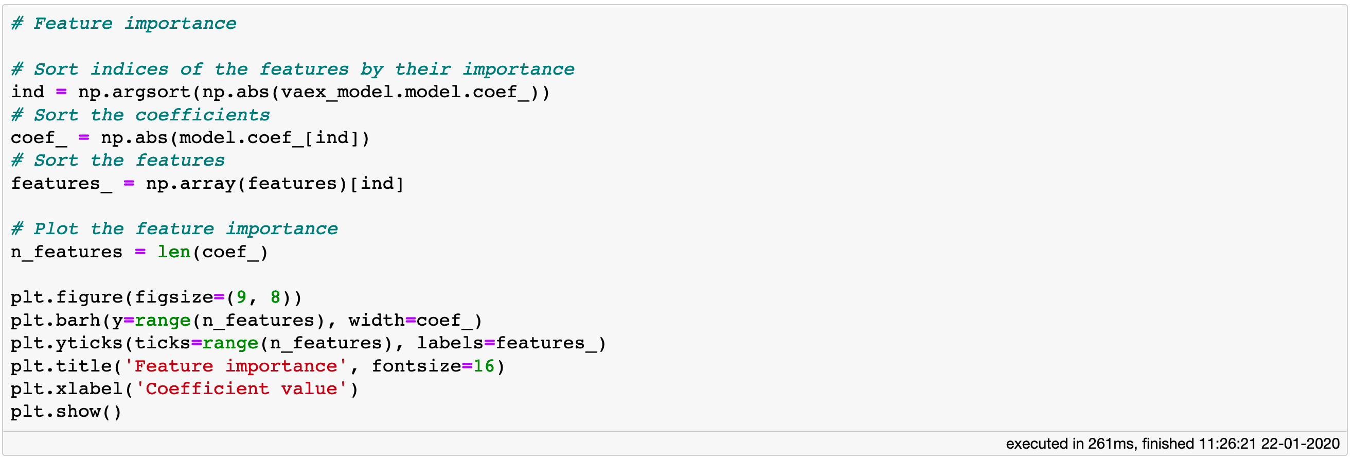
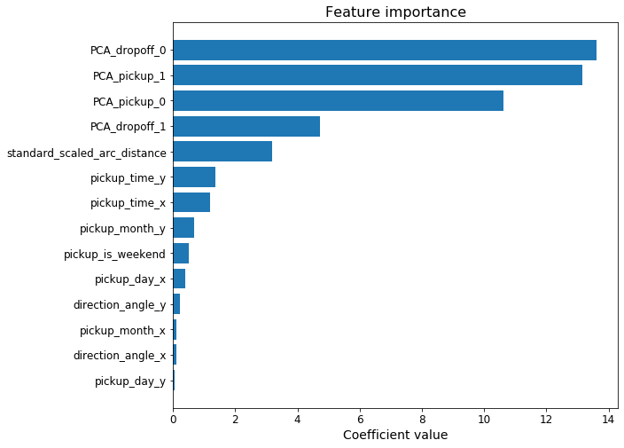The relative importance of the features used to train the model.

What about production?

Imagine that we manage to iron all the quirks out of our model, and that after a thorough validation it is ready to be put in production. In principle, this is quite easily done with Vaex. All that is required is for one to store the state in the production environment. The state can than be easily applied on an incoming Vaex DataFrame, and the predictions will be readily available.

Recall that the state not only memorizes all virtual columns that were created, but also which filters were applied. So, if one would query a prediction for a sample which would be filtered out if it was part of the training set, at prediction time it would also be filtered out, and thus that sample would “disappear”. In reality, samples can not just go missing, and many production cases require that we always return at least some kind of a prediction, no matter the query.

To overcome this hurdle, we can make use of the fact that in Vaex, a filtered DataFrame actually still contains all of the data, plus an expression that defines which rows are filtered out, and which are kept. While in other common libraries such as Numpy and Pandas one can only filter out more rows, in Vaex one can actually get rows back by using the “or” operator in a filter.

Let’s implement this idea for our problem. We add a variable called “production” to the training DataFrame and set its value to False. Then, we add an additional filter, which in this case is just the value of the variable. However, now we use the “or” instead of the default “and” operator which is used in cases like df3 = df2[df2.x < 5]. The idea is simple: if this last filter is set to False, it will have no effect on any other filters since its mode of operation is ”or”. If it is set to True however, which can be done by modifying the value of the “production” variable, it will invalidate all other filters, and thus any data point can pass through.

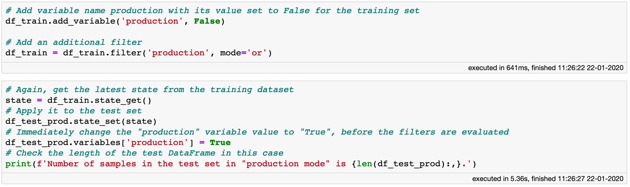An example of how filters can be enabled or disabled with a help of a variable in a Vaex DataFrame.

The code block above shows how we can include and modify the “production” variable such that the filters are disabled when needed. We can easily confirm that in this case, the test DataFrame contains as many samples as it did when we preformed the train/test split, with a prediction for each of them. Calculating the mean absolute error in this case gives us a higher result of 13 minutes, which is not surprising given that the model is ill trained to provide predictions for the many outliers or erroneous samples that are now part of the test set.

Our vision of the future

I hope I managed to show you how easy and convenient it is to create a machine learning pipeline using Vaex, even when the training data numbers over a billion samples and takes over 100 GB of disk space. I am sure you will find much more creative ways of using Vaex to improve the model presented in this article, as well as create many new ones for various other problems and use cases.

We, the Vaex team, believe in a future in which data science and machine learning can be down both conveniently and efficiently, even for “big” data, with tools that are free and open-source. We aim to make Vaex better integrated with the pillars of the Python data science stack, and are putting considerable efforts in bringing Vaex and scikit-learn closer together. Stay tuned, there are definitely more exciting things coming this way!

Happy data sciencing!